Visual Encoding Channels: Position, Length, Color and More
 By Tony Astor ·

Visual Encoding Channels
Visual encoding maps data values to visual properties—position, length, angle, area, color, shape, and texture—so charts can be read accurately. Position on a common scale is the most precise channel, followed by length, angle, area, and color. Matching channels to data types and communication goals produces faster, more accurate reading.
Table of Contents
- Visual Encoding Basics
- Spatial Position
- Line Length
- Slope and Direction
- Angle and Slice Size
- Area and Volume
- Color Hue
- Color Intensity and Shade
- Symbol Shapes and Size
- Pattern and Texture
- Grouping and Proximity
- Connecting Lines and Enclosure
- Visual Accuracy Hierarchy
- Inclusive Color Choices
- Smart Channel Selection
Visual Encoding Basics
Visual encoding is the process of mapping data values to visual properties such as position, length, color, and shape. Each property acts as a channel that carries information from the data domain into the perceptual domain. When a data point is assigned to a mark—a point, line, or bar—and that mark’s visual characteristics are systematically varied in proportion to the data values, the result is a graphic that the human visual system can interpret without conscious calculation. The brain can compare lengths, detect differences in position, and group similar colors almost instantaneously.
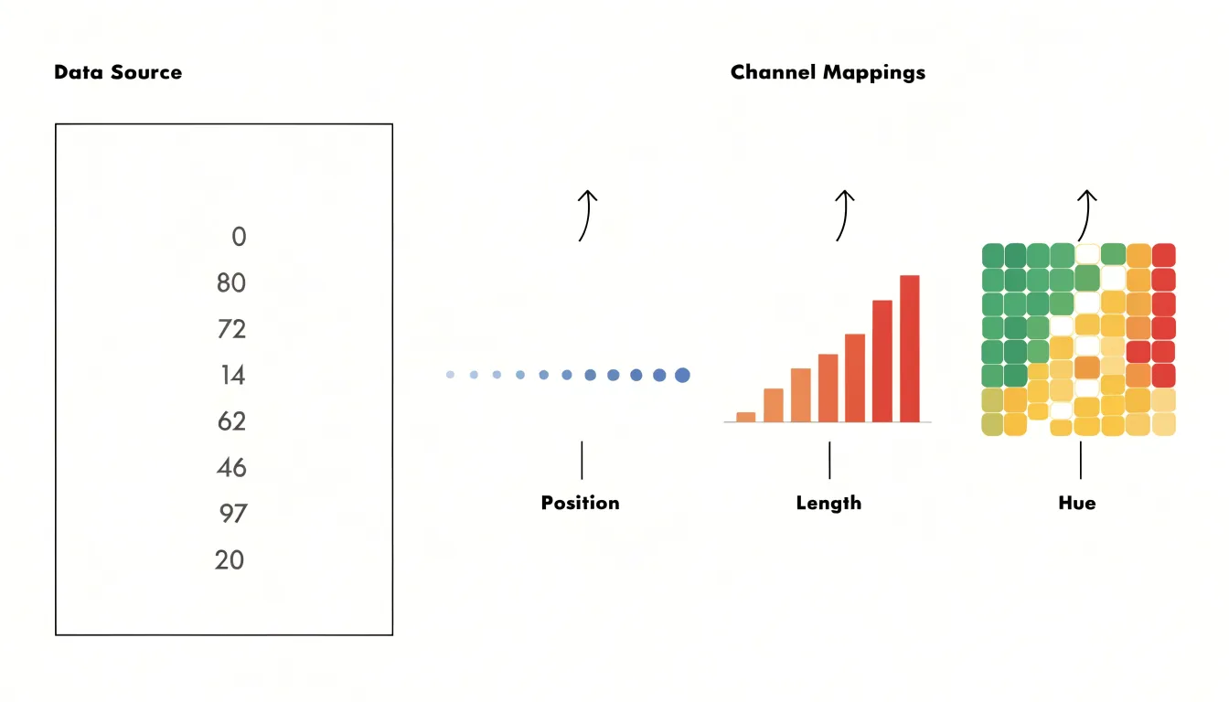
The core mechanisms of visual encoding rely on three key principles:
- Match the channel to the data type: Quantitative values are best represented by channels that convey magnitude, such as position on a common scale or length, while categorical data are better served by channels like shape or color hue.
- Preserve order and proportionality: The encoding should ensure that perceived visual differences mirror actual data differences.
- Account for the limits of human perception: Some channels, like position, support finer discrimination than others, like area or color saturation.
By applying these principles, designers can transform raw numbers into visual marks that reveal trends, outliers, and relationships that would be difficult to discern from tables alone.
Spatial Position
Spatial position refers to the placement of marks along a common scale, such as a horizontal or vertical axis. Perceptual research consistently identifies it as the most accurately decoded visual channel available to chart designers. The eye and brain are exceptionally attuned to aligning objects and judging their relative locations against a shared reference. When two values are encoded as positions on the same axis, a reader can compare them by tracing a straight line from each mark to the scale.
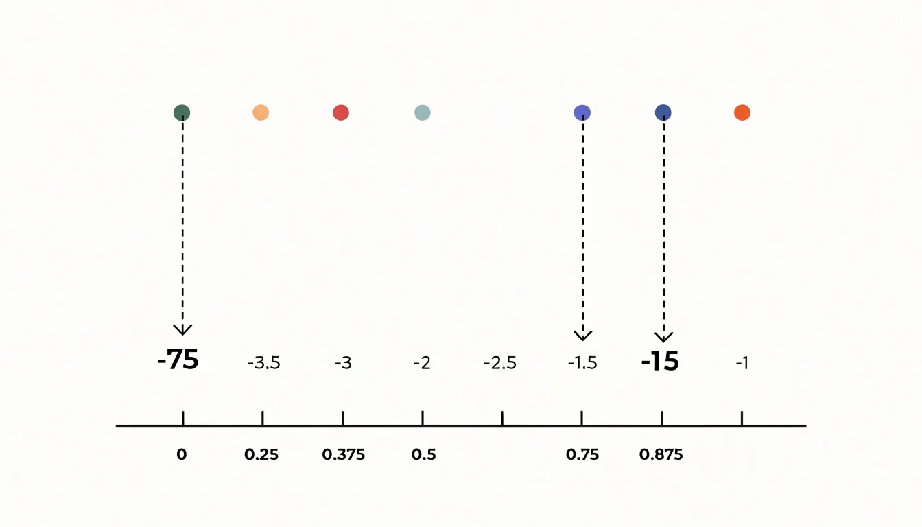
Experimental studies, notably the classic ranking work by Cleveland and McGill, found that position judgments produced the smallest errors of any tested encoding, outperforming length, angle, area, and color. Because position on a shared scale provides an explicit baseline, differences between values become simple distances along the axis rather than estimates of magnitude.
This encoding also stays robust when many marks are present, because each point retains a unique location that the eye can resolve individually. Scatterplots, dot plots, and line charts all anchor their data to position, and these forms remain reliable even at small sizes or with dense datasets. When a task requires precise comparison of quantitative values, placing marks along a common scale offers the highest fidelity reading the visual system can provide.
Line Length
Bar charts excel at communicating value differences because they encode quantity as length, one of the most accurate visual channels after spatial position. When a viewer compares two bars, they evaluate the distance from a shared baseline to the end of each bar, relying on the visual system’s strong sensitivity to extent and proportion. Because length judgments consistently outperform judgments of angle, area, or color saturation, the bar chart remains the default choice for comparing discrete categories.
The shared baseline is central to this clarity. Because every bar in a standard bar chart grows from the same starting line, differences in value appear directly as differences in how far each bar extends. A reader can look at two adjacent bars and immediately see which is longer, by how much, and how that gap relates to the total. This makes comparisons across unaligned categories straightforward: categories do not need to sit on a continuous axis, as each bar carries its own clear starting point.
Length also supports quick scanning across many categories. A long bar stands out against shorter neighbors, and rank order becomes visible at a glance. Subtle differences remain legible because the eye can compare stretches of line accurately, particularly when bars sit side by side. This combination of speed and precision makes bar charts effective for dashboards, reports, and exploratory analysis where readers need to spot the largest and smallest values and understand the gaps between them without careful measurement.
Slope and Direction
Slope and direction are intuitive visual channels for communicating how a quantity changes over time. When a line segment tilts upward from left to right, viewers immediately read that as an increase; a downward tilt signals a drop. This mapping mirrors everyday physical experience, such as climbing a hill or watching a value fall, allowing a well-drawn line chart to communicate the overall trajectory of a time series before a reader has processed any axis labels or numbers.
The angle of a segment encodes the magnitude of change: a steep slope indicates rapid change, while a shallow slope indicates slow change, allowing viewers to compare rates across different periods or series within the same chart. Direction adds a second layer, where rising, falling, or flat orientations correspond to growth, decline, or stability. When several segments are joined together, patterns such as acceleration, deceleration, and turning points emerge from the sequence of orientations alone.
Effective use of slope depends on consistent scales and enough horizontal space for angles to be readable. Compressed time axes can exaggerate or flatten perceived rates, so designers should keep the time interval proportional to the changes being shown. Annotations highlighting notable segments, such as a sharp rise or a prolonged decline, help direct attention to the most meaningful trends.
Angle and Slice Size
Pie charts encode data using angle and slice size, where each slice’s central angle is proportional to its share of the whole. The circular format naturally conveys a complete whole (100 percent), making pie charts effective for showing how individual categories contribute to a total when there are few categories and the proportions are distinctly different.
However, the perceptual system is less accurate at judging angles and areas than at comparing positions or lengths along a common scale. When slices are similar in size, differences become difficult to detect, and viewers may rely on cues like arc length or slice area, which can complicate perception. Small differences in angle are especially hard to discern, and the orientation of a slice within the circle can also affect judgments. Consequently, pie charts with many small slices or slices close in size can lead to misinterpretation.
Despite these challenges, pie charts remain popular in presentations and reports for communicating simple part-to-whole messages. To mitigate perceptual issues, limit the number of slices, order them logically, and label them clearly. When precise comparisons are needed, bar charts are more effective.
Area and Volume
Area and volume encodings map data values onto the physical size of shapes, and the way size grows with the underlying number determines whether readers judge the values accurately. When a circle’s area represents a value, the radius must scale with the square root of that value, because area grows with the square of the radius. If a designer instead scales the radius in direct proportion to the data, a value twice as large produces a circle with four times the area, exaggerating the underlying quantity. The same principle applies to rectangles and squares: if two rectangles encode values of 10 and 20 and the designer doubles both width and height, the larger rectangle covers four times the area for a two-to-one data ratio. The correct approach scales one dimension by the square root of the ratio, or adjusts width and height so their product matches the intended proportion.
Three-dimensional objects add further distortion. A value mapped to a sphere’s volume requires linear dimensions to scale with the cube root of the value. Double the data value and the diameter should grow by only about 26 percent; doubling every dimension produces eight times the volume, an error that compounds across a large range. Perceived size also depends on perspective, distance, and occlusion, making volume comparisons unreliable even when mathematically correct. Furthermore, readers tend to underestimate the volume of larger objects, adding a perceptual bias.
For two-dimensional shapes, compute the radius or side length from the square root of the value and state the encoding clearly. For three-dimensional visuals, use the cube root or avoid volume encoding altogether for precise comparisons. Where shapes sit side by side, a legend showing reference sizes at several known values helps readers calibrate their judgment.
Color Hue
Color hue is best suited to separating qualitative categories, because differences in hue are perceived as differences in kind rather than amount. When a chart assigns blue to one region and orange to another, or red to one product line and green to a second, the viewer reads those colors pre-attentively as labels. This makes hue a powerful tool for segmenting data into nominal classes such as region, department, customer segment, or experimental condition.
Unlike lightness or saturation, which naturally read as more or less, a set of distinct hues carries no built-in order. This makes hue ideal when categories are genuinely unordered and any apparent ranking would be misleading. If a legend pairs four colors with four regions, viewers will treat the regions as co-equal members of a set.
Designers can reinforce this reading by:
- Choosing hues of similar lightness and saturation across categories so no color stands out as heavier or more important.
- Keeping the number of hues modest so each remains clearly distinguishable.
- Avoiding colors that carry strong cultural or semantic associations, or that fall close together on the color wheel, since near-hues blur category boundaries.
Used with care, hue segments marks into clean, parallel groups while leaving questions of magnitude to channels better equipped to answer them.
Color Intensity and Shade
Color intensity and shade offer a direct way to encode a continuous numeric range. By varying saturation (the vividness of a hue) or brightness (how light or dark that hue appears), a designer creates a visual ramp that viewers read as a progression of magnitude. Light, desaturated tones sit naturally at the low end of the scale, while deeper, more saturated tones communicate higher values. This works because viewers intuitively associate darker, richer tones with denser, more concentrated quantities, making the encoding legible without requiring a legend lookup for every mark.
Sequential gradients serve data that moves in a single direction, from low to high. A typical sequential scale progresses through lightness steps within one hue or a narrow band of related hues, producing a smooth continuum that maps density levels, counts, or rates. Choropleth maps of population density demonstrate this well, as regions shade gradually from pale to deep as values climb. Because the transitions are continuous rather than stepped, viewers can estimate relative magnitudes by comparing shades side by side.
Diverging gradients extend this to data with a meaningful midpoint. Two sequential ramps are joined at a neutral, usually light, center, with each arm progressing toward its own saturated extreme. This structure suits values that fall above or below a reference point, such as temperature anomalies or profit and loss, letting viewers see both direction and distance from the baseline at a glance.
Symbol Shapes and Size
Symbol shapes separate categories on a map or chart without relying on color alone. Circles, squares, triangles, diamonds, and icons each carry an immediately recognizable identity, so a reader can tell at a glance whether a point represents a city, a factory, a weather station, or a hospital. Because shape differences survive grayscale printing, colorblind viewing, and small display sizes, they function as a robust categorical channel. Designers should choose visually distinct shapes, avoid overly intricate silhouettes that collapse at small scales, keep the number of shapes modest so the legend stays readable, and maintain consistent shape assignment across a series of figures.
Size, by contrast, encodes quantitative magnitude. Proportional symbol sizing scales the area of each glyph to match the represented value. As noted in the Area and Volume section, scaling by area rather than diameter is essential, and a legend with reference symbols helps readers estimate intermediate values. Size is best reserved for a single quantitative variable at a time, because overlapping size ranges are difficult to compare. Combining shape and size lets one symbol set communicate two dimensions at once, with shape sorting observations into categories and size expressing how much each observation represents.
Pattern and Texture
Pattern and texture give a chart an additional variable after position and color, distinguishing regions by the density and direction of surface marks. Cross-hatching builds tone through intersecting sets of parallel lines, using line angle and spacing to encode distinct categories without relying on hue. Stippling works through the accumulation of small dots, where denser clusters read as darker and sparser clusters as lighter. Both techniques separate regions while keeping the underlying geometry of the chart visible.
This is especially useful in monochrome and print formats, where color reproduction may be unreliable or reduced to grayscale. A map or stacked area chart that depends on subtle color differences can collapse into a single gray mass once printed, but varied hatching angles or dot spacing produce clear boundaries that survive photocopying, low-resolution output, and black-and-white reproduction.
Because pattern is applied within existing chart regions rather than layered on top as separate elements, it increases information density without adding clutter. The key is calibration: line spacing and dot size should be fine enough to read as a consistent tone at normal viewing distance, yet coarse enough that individual marks remain visible up close. Overly dense patterns shimmer and obscure the data, while overly loose ones fragment into isolated marks that no longer read as a unified surface.
Grouping and Proximity
The Gestalt principle of proximity states that elements placed close together are perceived as belonging to the same group, while elements separated by distance read as distinct. Because this perceptual tendency operates pre-attentively, designers can cluster related points so that the structure of the data becomes apparent at a glance, without requiring labels or explanatory text.
In practice, proximity governs much of the layout work in charts and diagrams:
- Scatterplots naturally form clumps where values concentrate, revealing the underlying distribution.
- Small multiples, matrix layouts, and faceted displays rely on spacing to signal which panels belong to the same category and which stand apart.
- Whitespace announces conceptual boundaries through generous gaps, while tight arrangements suggest shared identity. Adjusting the spacing between groups—the proximity ratio—tunes how strongly the segmentation reads.
Hierarchical structure emerges when proximity operates at multiple scales. Tight spacing binds points into small subgroups, moderate spacing combines those subgroups into larger clusters, and wide margins separate major categories. This nesting lets viewers traverse the visual hierarchy in either direction, zooming in on individual cases or stepping back to compare whole segments.
The main risk is ambiguity. When spacing is inconsistent or cluster boundaries fall in arbitrary places, viewers may perceive groups that do not exist or miss groups that do. Testing the layout with fresh eyes ensures that gaps correspond to meaningful divisions.
Connecting Lines and Enclosure
Connecting lines and enclosure make relationships and groupings explicit when spatial arrangement alone is insufficient. A connecting line, or link, is drawn between two marks to indicate a relationship such as a network edge, a flow, or a hierarchy. Its visual properties encode specific attributes of that relationship:
- Position, length, and curvature: Straight lines suggest direct connections, while curved or orthogonal lines route around obstacles.
- Line thickness: Represents the strength or volume of the connection.
- Line style: Solid, dashed, or dotted lines distinguish categories or states.
- Arrowheads: Add directionality, turning a link into a directed edge that shows flow or dependency.
When many links are drawn together, they form a network diagram that reveals topology—clusters, hubs, bridges, and bottlenecks—that would be invisible if the nodes were shown alone.
Enclosure works by drawing a boundary shape—a simple outline, a shaded region, or a tight hull—around a set of marks to indicate group membership. It is particularly effective for highlighting subsets within a larger display, because the eye treats the visual container as a single object. In hierarchical data, nested enclosures represent levels of grouping, with each boundary denoting a parent category. Overlapping boundaries show shared membership, while separate boundaries show distinct groups.
Used together, lines show pairwise relationships while enclosure shows set membership, allowing designers to depict network hierarchies (links within nested groups), flow paths (directed links crossing group boundaries), and structural relationships across enclosed regions.
Visual Accuracy Hierarchy
A visual accuracy hierarchy ranks encoding channels by how precisely people can read values from them:
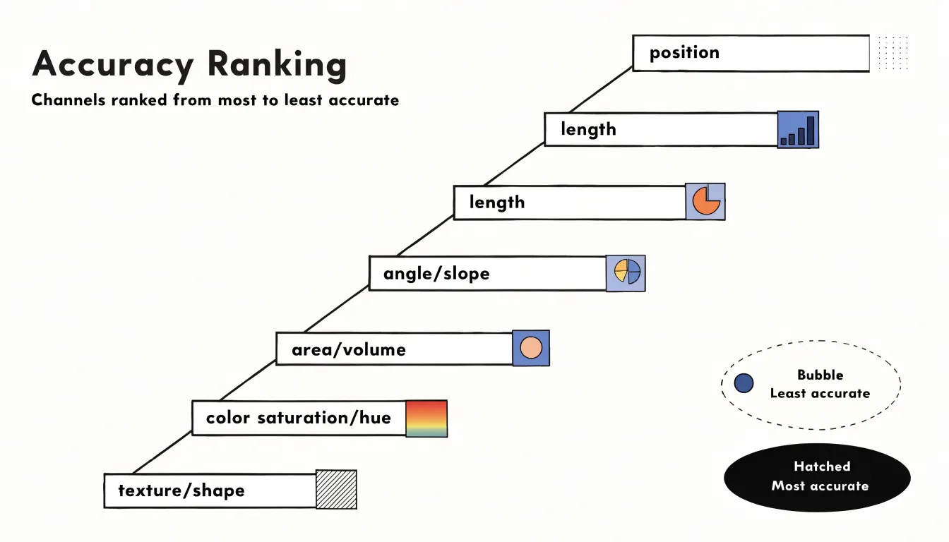
- Position on a common scale and position on non-aligned scales: Placing marks along a shared axis allows the finest-grained judgments (e.g., dot plots, scatterplots).
- Length: Comparing the extent of bars anchored to a common baseline is highly reliable.
- Angle and slope: Effective for general trends and proportions, but require more perceptual effort, which is why pie charts trail bar charts in accuracy.
- Area and volume: Judging the relative size of 2D and 3D shapes grows increasingly unreliable as differences shrink.
- Color saturation and color hue: Useful for rough groupings or categories, but poor at conveying exact magnitudes.
- Texture, shape, and motion: Best suited to labeling or attracting attention rather than precise quantitative comparison.
This ordering is a practical guide rather than an absolute law. A chart comparing sales figures will serve readers better with position or length than with color saturation. When a lower-ranked channel must be used, pairing it with a higher-ranked channel—such as adding direct labels or aligning bars to a baseline—helps compensate. When evaluating competing designs that convey the same data, the one relying on a higher-ranked channel usually produces faster, more accurate reading.
Inclusive Color Choices
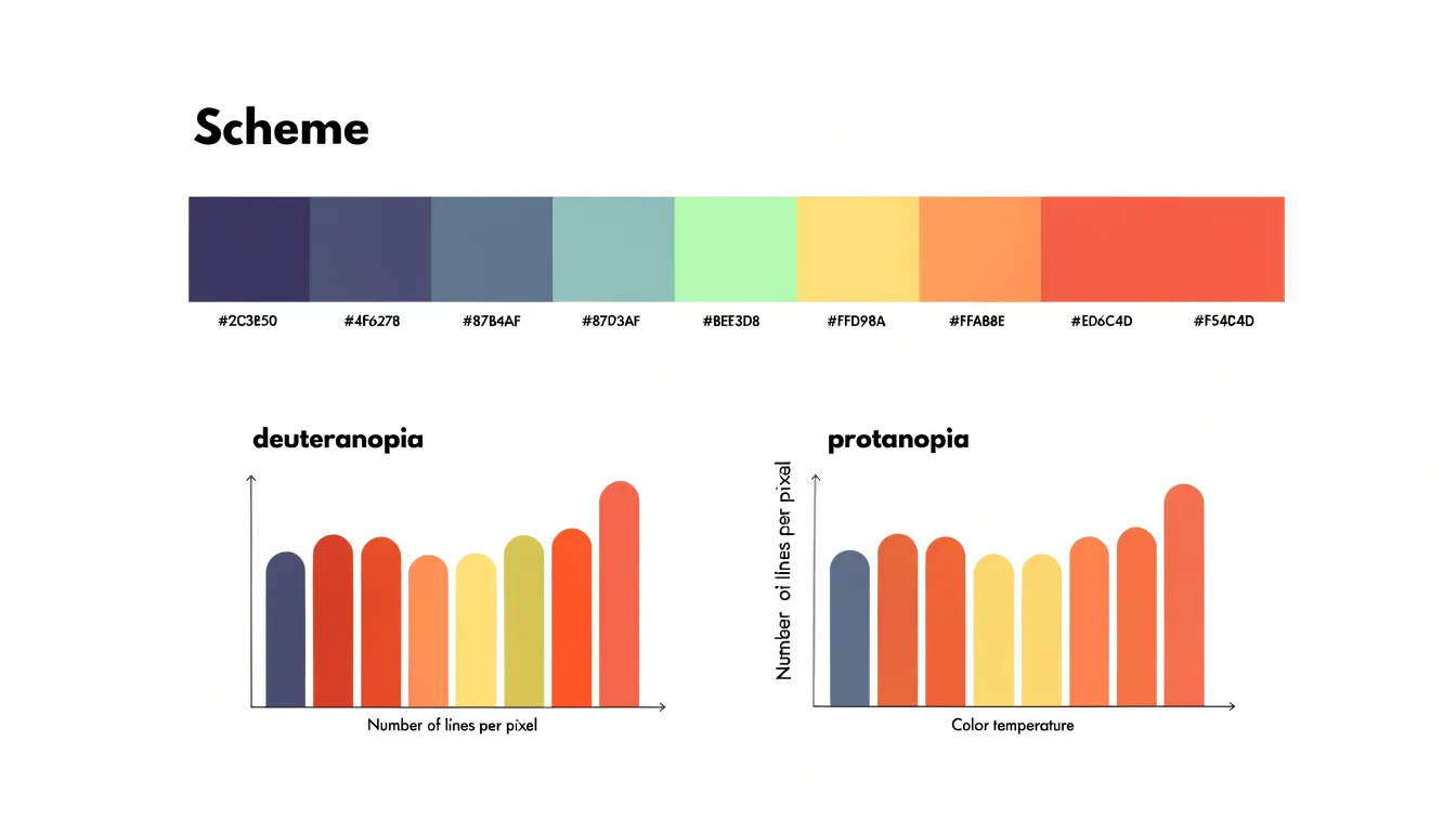
Roughly one in twelve men and a smaller proportion of women experience some form of color-vision deficiency, most commonly in the red-green range. A palette that looks distinct to the designer can collapse into near-identical muddy tones for these readers. Accessible palette design addresses this by selecting hues that remain separable under common forms of color blindness.
The Okabe-Ito scale, developed by Masataka Okabe and Kei Ito, is a widely adopted starting point. It offers eight colors chosen to stay distinguishable for deuteranopes, protanopes, and tritanopes alike. Relying on variations in lightness and hues outside the red-green confusion zones, it pairs warm orange and vermilion with sky blue, bluish green, and yellow, providing a solid accessible default without requiring a custom audit for every project.
Beyond palette selection, redundant encoding reinforces color with a second, independent visual cue so meaning survives even when hue perception fails:
- Pairing each color with a distinct symbol shape or marker.
- Varying line styles (solid, dashed, dotted).
- Applying direct labels to series rather than relying on a legend.
- Adding texture or pattern fills to areas.
- Varying lightness across sequential scales, since luminance differences remain readable across most color-vision deficiencies.
Finally, designers should test graphics by simulating protanopia and deuteranopia in browser tools or image editors, or by converting charts to grayscale to confirm that key distinctions persist.
Smart Channel Selection
Selecting the right combination of channels follows a four-step process:
- Inventory your data’s attributes: Identify whether each variable is categorical, ordinal, or quantitative, and note its range, precision, and natural ordering. Align the channel’s strengths with the data structure—using position, length, or angle for quantitative data, and color hue, shape, or spatial grouping for categorical data.
- Articulate your communication goal: Match the channel emphasis to the task. Use position and length for comparing categories; position, slope, and color lightness for trends over time; position on two axes with color or size as a third channel for correlations; and area or angle (or position and length for higher precision) for part-to-whole relationships.
- Combine channels without conflict: Assign the most accurate channel (typically position) to the most important variable, and less precise channels (like color or shape) to secondary variables. Avoid using the same channel for multiple variables unless one is clearly secondary—for instance, reserve color hue for categories and use lightness or size for a quantitative measure rather than encoding both with hue.
- Test against viewing tasks: Verify that viewers can quickly find the largest value, compare groups, and see the overall pattern, adjusting channel assignments if necessary.
Frequently Asked Questions
What is visual encoding in data visualization?
Visual encoding is the process of mapping data values to visual properties such as position, length, color, and shape. These properties act as channels that carry information from the data domain into the perceptual domain.
Which visual channel is most accurate for reading values?
Spatial position on a common scale is the most accurately decoded visual channel. Studies by Cleveland and McGill found that position judgments produced the smallest errors, outperforming length, angle, area, and color.
Why are bar charts good for comparing categories?
Bar charts encode quantity as length and use a shared baseline, so differences in value appear directly as differences in how far each bar extends. Length judgments consistently outperform judgments of angle, area, or color saturation.
When are pie charts appropriate to use?
Pie charts are effective for showing part-to-whole relationships when there are few categories and the proportions are distinctly different. To reduce perceptual issues, limit the number of slices, order them logically, and label them clearly; bar charts are more effective when precise comparisons are needed.
How should you scale circles or symbols to represent data values?
When a circle’s area represents a value, the radius must scale with the square root of that value. Scaling the radius directly in proportion to the data exaggerates the quantity, and for three-dimensional visuals, linear dimensions should scale with the cube root or volume encoding should be avoided for precise comparisons.
How can I make charts accessible for people with color-vision deficiency?
Use accessible palettes such as Okabe-Ito and reinforce color with redundant encoding like distinct shapes, line styles, direct labels, texture, or lightness differences. Designers should also test graphics by simulating protanopia and deuteranopia or converting charts to grayscale, since roughly one in twelve men and a smaller proportion of women experience some form of color-vision deficiency.
Tony Astor
Tony writes about data visualization and the tools people use to build charts and dashboards. More about Data Illustrator