Violin Plot: What It Shows That a Box Plot Doesn't
 By Tony Astor ·
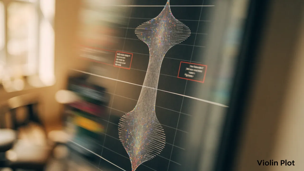
Violin Plot
A violin plot is a data visualization that mirrors a kernel density estimation curve around a central axis, forming a violin-like shape where wider sections indicate densely packed values and narrow sections indicate sparse regions. It reveals skewness, multimodality, and concentration that box plots hide, making it useful for comparing distribution shapes across groups.
Table of Contents
Box Plot
A box plot summarizes a dataset’s distribution through five statistics: the minimum, first quartile (Q1), median, third quartile (Q3), and maximum. These numbers divide the data into four sections, each containing approximately 25% of the observations. The central box spans from Q1 to Q3, representing the interquartile range (IQR), which captures the middle 50% of the data. A line inside the box marks the median. Whiskers extend from the box to the minimum and maximum values—often defined as the most extreme observations within 1.5 times the IQR from the quartiles—with points beyond these limits plotted individually as outliers.
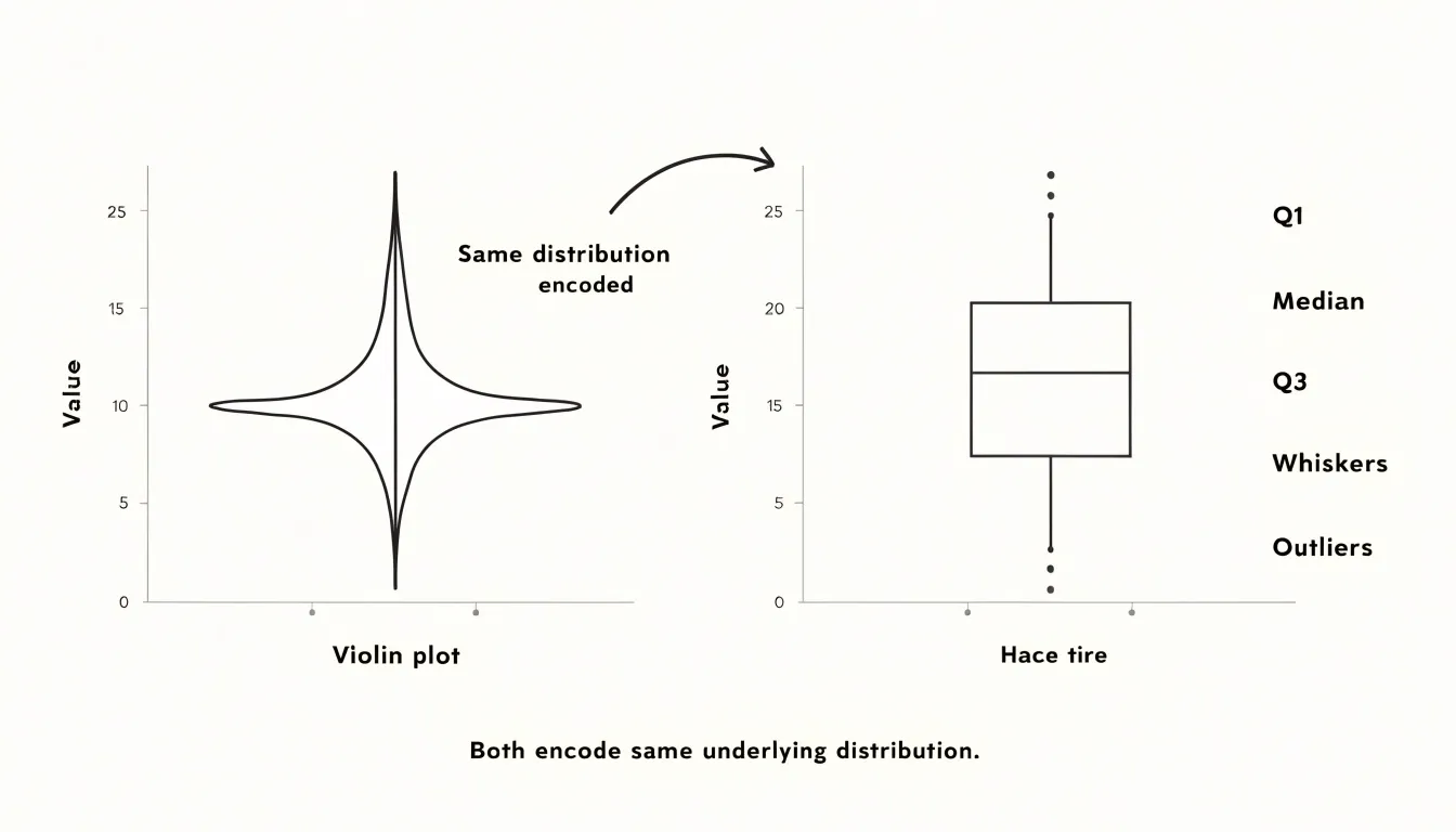
When comparing multiple groups, box plots align these five-number summaries side by side on a common scale for quick comparisons of central tendency, spread, and skewness. One can immediately see which group has the highest median, the widest IQR, or outliers. The shape of the box and relative whisker lengths also reveal skewness: a longer upper whisker suggests a right-skewed distribution, a longer lower whisker indicates left skew, and an off-center median within the box hints at asymmetry.
Box plots are especially useful for large numbers of groups or non-normally distributed data because they rely on robust statistics like the median and IQR without making distributional assumptions. However, they do not show the exact shape of the distribution or the presence of multiple modes, which is where violin plots complement them by adding a density estimate.
Violin Plot
A violin plot earns its name from the symmetric, violin-like silhouette formed by mirroring a kernel density estimation (KDE) curve around a central axis. The KDE places a small, smooth bump over every observed data point and sums those bumps into a single continuous curve. In the resulting profile, wider sections indicate ranges where observations are densely packed, and narrower sections indicate sparse regions.
Because the curve traces the full shape of the data, it exposes features that summary statistics hide:
- Skewness: A long, thin tail stretching toward high or low values signals that the distribution leans in that direction, which a simple mean and standard deviation cannot convey.
- Multimodality: Multiple peaks along the curve point to clusters within the data, suggesting distinct subgroups or a mixture of populations bundled into one category.
- Concentration: A broad, flat profile shows that values are spread out fairly evenly, while a tall, narrow bulge indicates strong concentration around a central value.
The density curve also reveals how much mass sits in the shoulders and tails of the distribution, indicating the spread beyond the central range. Showing concentration, skew, and clustering in one shape makes the violin plot especially useful for comparing groups side by side, where differences in shape and density highlight patterns that averages alone would mask.
Bimodal Data
Because a box plot reduces a distribution to five summary statistics, it carries no information about where observations cluster between those landmarks. When a dataset contains two or more subgroups, this compression can be misleading. Two datasets with very different shapes—such as a unimodal distribution and a bimodal one constructed so their quartiles coincide—can produce identical box plots with the same median, IQR, and whisker span.
Violin plots address this limitation directly. In a bimodal dataset, the violin plot reveals two distinct bulges separated by a narrow waist, making subgroups immediately visible. The viewer can judge the relative size of each mode, their separation, and the depth of the valley between them.
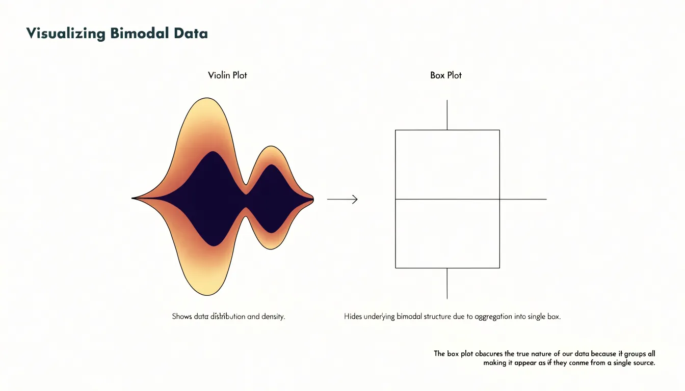
Exposing multiple peaks is valuable whenever observations may come from mixed populations, such as measurements pooled across conditions, sites, or instrument settings. Where a box plot suggests a single homogeneous sample, the violin plot shows the internal structure, preventing inappropriate summary statistics and pointing toward subgroup analysis before modeling begins.
Density Width
Reading a violin means scanning its contour like a distribution curve turned on its side, with the widest spans marking the most common values. In most implementations, the two sides of the violin are mirror images, so the full width at a given height is twice the estimated probability density at that point. A single prominent bulge suggests a unimodal distribution, while a violin that tapers quickly from a wide base signals a heavy concentration near the extremes of the observed range.
Width comparisons across separate violins require care because scaling depends on the kernel bandwidth and normalization method:
- Equal maximum width: When every violin is scaled to the same maximum width, widths can be compared across groups as relative densities.
- Equal area: When violins are scaled to equal total area, width conveys less about absolute frequency and more about shape.
Checking the plotting defaults or documentation clarifies which convention applies and how confidently a reader can infer frequency from the contour.
Central Tendency
Small markers embedded inside a violin plot—a dot, a short horizontal bar, or a miniature box plot—anchor the viewer’s attention to the distribution’s central tendency.
The most common marker is the median, typically shown as a white dot or horizontal line. The median’s position relative to the widest section reveals skewness: if it sits near the bulge, the distribution is roughly symmetric; if it lies toward one tail, the data are skewed in the opposite direction.
The mean is sometimes added as a small cross or differently colored dot. Comparing the mean and median within the same violin shows the influence of outliers: when the mean is pulled away from the median toward a long tail, extreme values are distorting the average. A mini box plot inside the violin adds quartiles and whiskers alongside the density curve. When comparing multiple violins side by side, the eye can quickly scan these markers across categories to detect shifts in central value.
Skewness
With the variable of interest on the vertical axis and density mirrored horizontally, skewness appears as an uneven vertical bulge:
- Right-skewed: The widest part of the violin sits low and tapers into a long, thin neck reaching upward; most values cluster near the bottom with a sparse tail of larger values extending toward the top.
- Left-skewed: The bulge sits high and the taper descends, with a thin tail of small values pulling downward.
In a box plot, skewness is implied indirectly through the median’s position and whisker lengths—cues that require interpretation and can be muted when whiskers are drawn to fixed multiples of the IQR. The violin makes skewness spatial and immediate: the bulge is the mode region, the taper is the tail, and the vertical drift is the skew. Analysts can scan a row of violins and spot which distributions lean right or left before running any formal test of asymmetry.
Outliers
Outliers in a violin plot appear as individual dots along the vertical axis, separated from the main density body. The distance between an outlier marker and the edge of the density body communicates how far that observation departs from the typical range.
As the density curve approaches these extremes, it tapers toward a narrow tip. Outlier markers often sit just beyond that taper where the KDE carries very little mass. This helps distinguish a genuine extreme from a long tail, as the curve shows how quickly density falls away before the isolated point appears.
When several violins sit side by side along a shared scale, a cluster of extreme values in one category is easy to spot next to categories with none, showing which groups carry unusual observations and whether those extremes are symmetric or one-sided.
Sample Size
Kernel density estimation depends directly on how many observations are available. With a large sample, individual probability bumps overlap densely, and the outline reflects genuine structure, including secondary modes or gradual shoulders. With a small sample, each observation carries substantial weight and the smoothing bandwidth spans wide gaps between points, drawing a curve through regions where no data exist. A violin drawn from a dozen values can look deceptively polished, implying a level of detail the data cannot support.
Small samples also create artifacts at the extremes. KDEs taper gradually toward the tails, which can suggest that extreme values extend farther than any actual observation or that the distribution has a smooth boundary where the data simply stop. Isolated points far from the main cluster may generate small bumps that look like meaningful subgroups when they are merely single observations.
Sample size should therefore be treated as part of the visual encoding. Readers should check the number of observations behind each violin or compare the density outline against an overlaid strip or dot plot. Analysts should report sample sizes alongside the plots or restrict density estimation to groups large enough to support it.
Grouped Violins
Placing multiple violin plots along a shared categorical axis against the same vertical scale allows viewers to read differences in density shape, spread, and central tendency horizontally. This side-by-side arrangement preserves the shape information that a bar chart of means discards.
Shared axes also support direct judgments of overlap: where two violins occupy the same vertical band, their groups share similar values; where one extends well above or below its neighbors, the difference stands out as a visible asymmetry. Grouping can be extended by placing violins adjacent within categories defined by a second factor, allowing density comparisons across two dimensions at once. When labels are clear and the number of groups stays moderate, grouped violins communicate distributional differences to audiences that may not read statistical summaries fluently.
Split Violin
A split violin divides the standard violin down the middle, placing one category’s density curve on one side of the central axis and a second category’s curve on the other. The division can run vertically (left versus right) or horizontally (top versus bottom). Because both halves share the same scale and axis position, the viewer’s eye can travel directly across the center line to compare where each distribution is thickest, how far each tail extends, and whether medians and quartiles align or diverge.
Because both groups occupy the footprint of one ordinary violin, a split violin delivers a binary comparison in roughly half the space of two side-by-side violins. On dashboards where plot area is scarce, a grid of split violins across several categories or time periods can show a treatment-versus-control or before-versus-after contrast for every group without doubling the number of plots. Furthermore, small differences in spread or skew are easier to perceive when both halves meet at the same axis than when they sit in separate panels. The format works best when the two categories form a natural pair, use consistent color for each side, and maintain a readable combined shape.
Bandwidth
The kernel bandwidth parameter controls the width of the smoothing window around each observation when computing the density estimate, determining how much neighboring observations bleed into one another:
- Small bandwidth: Produces a narrow kernel where each point contributes to a tight region around itself. The curve follows the raw data closely with sharp peaks and deep valleys, revealing fine structure like secondary modes and shoulders. However, random sampling noise gets rendered as real features, making the plot look jagged.
- Large bandwidth: Spreads each observation over a wider range, filtering noise into a smoother curve that emphasizes major features. However, genuine detail can be flattened, and distinct clusters may merge into a single broad mound.
Bandwidth is often chosen using rules of thumb, such as Silverman’s rule, or by cross-validation, which many plotting libraries tune automatically. Analysts exploring a distribution typically try several bandwidth values side by side: features that remain stable across settings are more likely to be real, while those that appear or vanish are usually smoothing artifacts.
Interpretation Pitfalls
Several recurring mistakes can distort conclusions drawn from violin plots:
- Confusing width with sample size: A wide bulge indicates relative concentration within a distribution, not total sample size. A violin built from 50 points and one built from 5,000 can display identical silhouettes. Always check accompanying text or axis annotations for actual sample counts before judging precision or effect size.
- Over-interpreting smoothing artifacts: Overly high bandwidths can flatten secondary modes or sharp boundaries and exaggerate or truncate low-density tails, while overly narrow bandwidths manufacture spurious bumps from noise. Treat minor wiggles in an outline with skepticism unless corroborated by a rug plot of individual data points.
- Ignoring tail trimming and mismatched settings: Trimmed tails can hide outliers and understate the data’s range, while differing bandwidths across groups make their shapes incomparable. Check methodology notes for bandwidth selection and tail handling, and pair the violin with a box plot or raw data overlay for context.
Box Plot Overlay
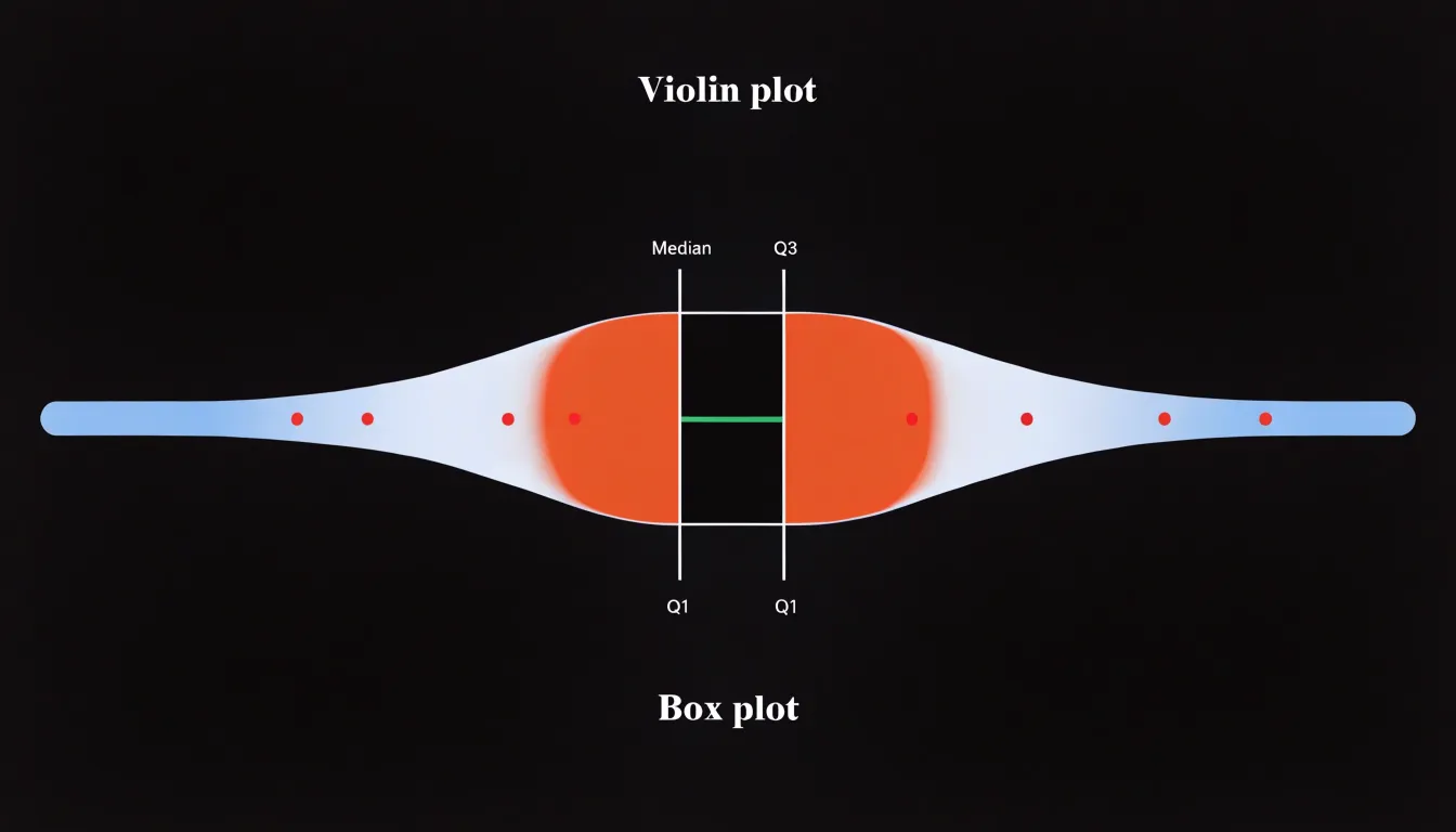
Embedding a narrow box plot centered inside a violin plot combines smooth density estimation with exact summary statistics. The outer violin reveals multimodality and skewness, while the inner box plot marks the exact median, quartiles, and whisker extremes that a violin alone does not clearly convey. Additionally, the box plot’s whiskers help identify outliers that might be obscured in the tapering density curve. This overlay is straightforward to implement in libraries such as ggplot2 or seaborn and has become a standard technique in exploratory data analysis.
Dashboard
When choosing between standard box plots, violin plots, or hybrid overlays, match the chart to your audience’s statistical literacy and the reporting context:
- Box plots: Familiar to most analysts and compact enough to remain readable across many groups. Use them for quick comparisons of central tendency and spread, or for audiences new to data visualization.
- Violin plots: Best for exploratory analysis or presentations where distributional shape, skewness, and multiple peaks matter, provided the audience can interpret density curves and sample sizes are sufficient, as violins become cluttered when too many groups are plotted.
- Hybrid overlays: Retain familiar quartile summaries while adding distributional detail, making them effective for mixed audiences.
Frequently Asked Questions
What is a violin plot and how is it different from a box plot?
A violin plot mirrors a kernel density estimation curve around a central axis, forming a violin-like silhouette where wider sections show densely packed observations and narrower sections show sparse regions. It complements a box plot by showing the full distribution shape, including skewness and multimodality, while a box plot summarizes data with five statistics.
How do you read the width of a violin plot?
Read the contour like a distribution curve turned on its side, with the widest spans marking the most common values; in most implementations the two sides are mirror images, so the full width is twice the estimated probability density. Width comparisons across violins require care because scaling depends on kernel bandwidth and normalization method, such as equal maximum width versus equal area.
What does a bimodal violin plot show?
In a bimodal dataset, the violin plot reveals two distinct bulges separated by a narrow waist, making subgroups immediately visible. The viewer can judge the relative size of each mode, their separation, and the depth of the valley between them.
Does a wider violin plot mean a larger sample size?
No. A wide bulge indicates relative concentration within a distribution, not total sample size, and a violin built from 50 points and one built from 5,000 can display identical silhouettes. Check accompanying text or axis annotations for actual sample counts before judging precision or effect size.
How does sample size affect a violin plot?
With a large sample, individual probability bumps overlap densely and the outline reflects genuine structure, including secondary modes or gradual shoulders. With a small sample, the smoothing bandwidth spans wide gaps between points and can draw a curve through regions where no data exist, so a violin from a dozen values can look deceptively polished.
What does bandwidth do in a violin plot?
Bandwidth controls the width of the smoothing window around each observation. A small bandwidth reveals fine structure like secondary modes and shoulders but can render random sampling noise as real features, while a large bandwidth smooths noise but can flatten genuine detail and merge distinct clusters into a single broad mound.
Tony Astor
Tony writes about data visualization and the tools people use to build charts and dashboards. More about Data Illustrator