Types of Charts: A Complete List With Uses
 By Tony Astor ·
Types of Charts
Charts fall into types chosen by data and purpose: bar charts compare discrete categories, line graphs track trends over time, pie charts show part-to-whole proportions, histograms display continuous distributions, and scatter plots reveal relationships between two variables. Area, bubble, box plot, heat map, treemap, waterfall, Sankey, choropleth, funnel, and candlestick charts each serve specialized comparisons.
Table of Contents
Bar Charts
Bar charts compare discrete categories using rectangular bars whose lengths encode values. Vertical bar charts (often called column charts) place categories along the horizontal axis and values along the vertical axis; this works well when category names are short and the audience reads comparisons left to right. Horizontal bar charts flip this arrangement, giving long category labels room to breathe. They are a strong choice for ranked lists, survey responses, or any dataset where names would otherwise crowd or rotate awkwardly along the bottom of the chart.
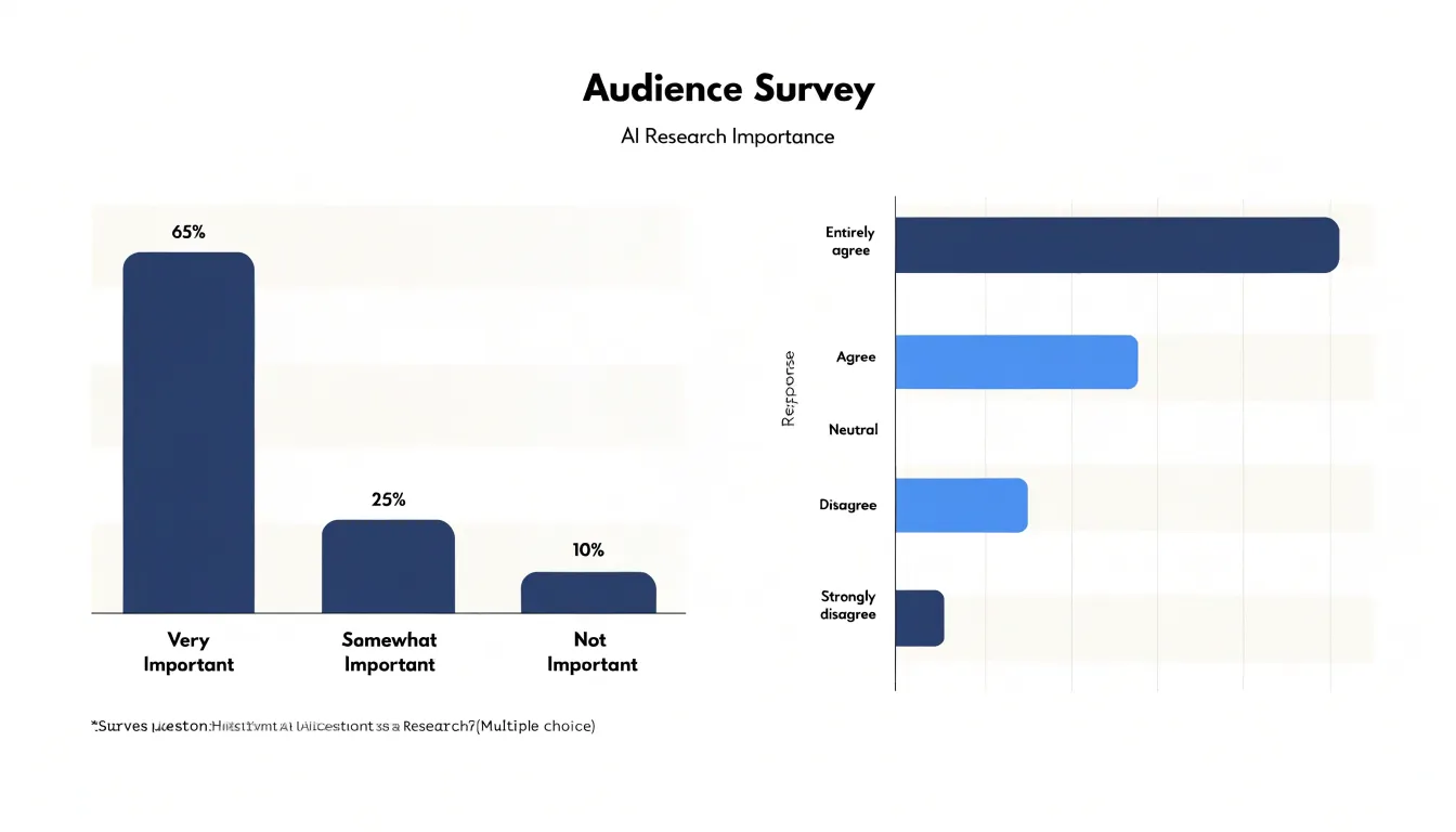
In both orientations, consistent spacing between bars separates each group visually, while the bar thickness signals that each rectangle stands for a single, self-contained quantity. Readers can scan the row of bars and immediately see which categories are larger, smaller, or roughly equal—a judgment that bar charts support more cleanly than almost any other form.
Baseline alignment is central to honest comparison. Because bars encode value through length, every bar must start from zero. Truncating the axis compresses differences or inflates small gaps, so the chart should begin at zero unless there is a clear, disclosed reason to do otherwise.
Several design choices keep bar charts readable:
- Gridlines and ticks: Keep them light enough to guide the eye without competing with the data.
- Labels: Use axis titles to state the units, place value labels at the end of each bar to reduce the need to trace back to the axis, and spell out category labels rather than abbreviating them into ambiguity.
- Ordering and scope: Order bars by value rather than alphabetically so readers see the ranking at a glance, and limit the number of categories to keep the chart legible.
- Title: Use a concise title that states the main takeaway.
Line Graphs
Line graphs track trends over continuous periods of time, making them well suited to time-series data where the sequence of observations matters. By connecting individual data points with straight or smoothed line segments, a line graph forms a continuous path that reveals how a value rises, falls, or holds steady across successive intervals. Unlike bar charts, which treat each category as an isolated unit, line graphs let viewers follow progression from one period to the next and read the overall shape of the data.
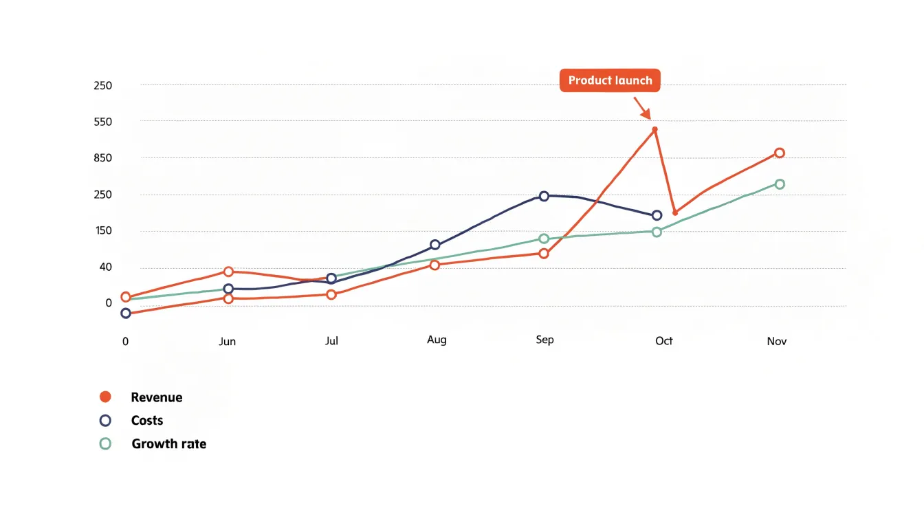
When plotting time-series data, the horizontal axis typically represents time at regular intervals—such as days, weeks, months, or years—while the vertical axis carries the measured value. Consistent interval spacing keeps the progression readable and prevents distortion of the trend. Multiple series can be plotted together using distinct line styles or colors to compare metrics, regions, or product lines over the same period. Analysts often annotate significant events, seasonal shifts, or milestones directly on the chart to explain visible changes in direction.
Effective line graphs emphasize directional patterns: sustained upward or downward movement, cyclical fluctuations, and sudden spikes or dips all show up through the slope and shape of the line. Common applications include monitoring revenue growth, tracking website traffic, and observing temperature changes. As with bar charts, light gridlines, clear axis labels, and a well-chosen scale help readers interpret magnitude accurately.
Pie Charts
Pie charts represent a whole divided into slices, where each slice’s central angle and area correspond to its share of the total. They communicate part-to-whole relationships at a glance, which makes them suited to static compositions such as budget allocations, market share breakdowns, or survey responses expressed as percentages. Because a pie chart always sums to 100%, viewers immediately see that the categories are mutually exclusive and collectively exhaustive.
Each slice’s angle must be calculated directly from its proportion of the total, so that a category representing a quarter of the whole occupies a quarter of the circle. Because readers judge slice magnitude by area and arc length simultaneously, starting the first slice at twelve o’clock and ordering slices clockwise from largest to smallest makes comparisons easier. Direct percentage or category labels placed on or beside each slice remove the need to estimate values from geometry alone.
The most common pitfall is overloading the chart with slices. Beyond about five to seven categories, small wedges become hard to distinguish and compare, and labels begin to collide. In such cases, consolidate the long tail of minor categories into a single combined slice and present the individual values in an accompanying table. Slices with very similar proportions are also hard to tell apart in a pie, and the format offers no good way to show change over time or to compare across multiple groups. Keep pie charts to a small number of clearly labeled slices for simple proportional data.
Histogram
A histogram shows the distribution of a continuous numerical variable by sorting observations into equal-width intervals called bins. To build one, span the range from the smallest to the largest value and divide it into consecutive intervals of identical width. Each observation falls into one bin, and the height of each bar reflects the count or proportion of observations in that interval. Because the bins are uniform and adjacent, the bars touch, signaling that the underlying variable is continuous rather than categorical.
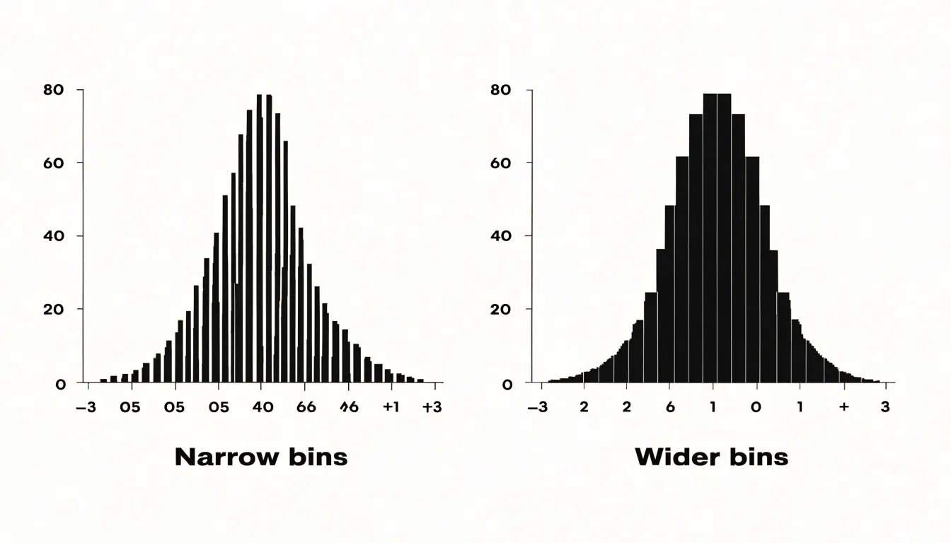
The choice of bin width shapes what the chart reveals:
- Narrow bins expose fine-grained detail and local bumps.
- Wider bins smooth out noise and emphasize the overall profile.
A sensible starting point uses enough bins to show structure without turning the chart into a spiky comb; analysts often try several widths before settling on one that shows the distribution clearly. Equal intervals keep the comparison fair, since every bar covers the same span of values and height differences map directly to frequency differences.
The resulting shape summarizes how the variable behaves before any formal statistical testing begins:
- Symmetry: A bell-like profile suggests values cluster around a middle region and taper off evenly on both sides.
- Skewness: A long tail stretching to the right or left means extreme values pull the distribution in one direction and the mean drifts away from the median.
- Peaks and central tendency: The tallest bars locate the mode (where values concentrate), the balance point of the bars approximates central tendency, and multiple peaks hint at subgroups or mixed populations within the dataset.
- Outliers: Isolated bars at either edge flag unusual values worth investigating.
Scatter Plot
A scatter plot maps two continuous numerical variables against each other, placing one on the horizontal axis and the other on the vertical axis. Each observation appears as a single point at the coordinates defined by its pair of values. This positional encoding reveals relationships that summary statistics like averages and totals can obscure by collapsing variation.
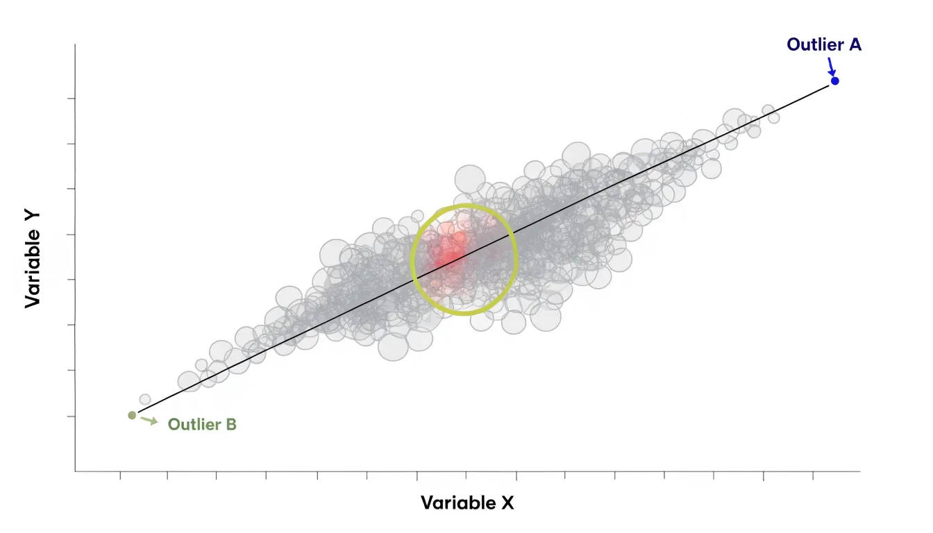
The most common pattern to look for is correlation:
- Positive correlation: Points trend upward from left to right, meaning higher values on one metric accompany higher values on the other.
- Negative correlation: Points slope downward, meaning increases in one variable correspond to decreases in the other.
- Strength: A narrow band of points suggests a strong association, while a wide, diffuse spread points to a weak one. Adding a trend line or regression curve helps clarify the direction and steepness of the relationship.
Beyond correlation, scatter plots expose clusters and outliers. Clusters—groups of points gathered in distinct regions—can reveal hidden segments, such as customers who behave alike or measurements taken under similar conditions. Outliers sit far from the main cloud and may represent data entry errors, rare events, or genuinely unusual cases deserving investigation.
To keep these patterns visible, match the axis scales to the data range, adjust point size and opacity when observations overlap, and consider using color to encode a third, categorical dimension.
Area Charts
Area charts build on line graphs by filling the space between the plotted line and the horizontal axis with a shaded region. Where a simple line emphasizes the path of a trend, the shaded area directs attention to magnitude, making area charts a natural fit for showing cumulative totals and volume over time. The visual mass of color corresponds directly to the quantity represented.
Area charts are especially useful when several series are stacked on a shared baseline. Stacking places each category on top of the ones below, so the total height of the combined region shows the overall cumulative figure at any point in time, while the individual bands show each component’s part-to-whole contribution. A product manager tracking revenue across several product lines, for example, can see both the growth of the overall business and the shifting share held by each line as the bands expand or contract.
Because the filled area carries meaning, use a consistent baseline to keep comparisons honest across the time series, and keep categories in a stable stacking order so bands do not jump position between points. Labels or a legend map colors to categories, while light gridlines anchor the eye without competing with the shaded regions.
Bubble Charts
Bubble charts extend the two-axis scatter plot by encoding a third quantitative variable through the size of each plotted marker. This lets analysts explore relationships among three metrics simultaneously without needing a third axis—for example, comparing countries by GDP per capita (x-axis), life expectancy (y-axis), and population (bubble size), or evaluating products by price, customer satisfaction, and sales volume.
Scale each bubble’s area—not its diameter—in proportion to the value it represents. Human perception tends to underestimate differences in area, and scaling by diameter exaggerates size differences. When area is scaled correctly, viewers can compare bubble sizes with reasonable accuracy.
Because bubble size is a less precise visual encoding than position, bubble charts work best for highlighting broad patterns and outliers rather than exact comparisons. Overlapping bubbles can also obscure data when points cluster together or sizes vary widely. Use transparency, distinct colors, and interactive tooltips to keep overlapping points readable.
Box and Whisker Plots
A box and whisker plot (or box plot) condenses a dataset into a compact five-number summary that describes both center and spread:
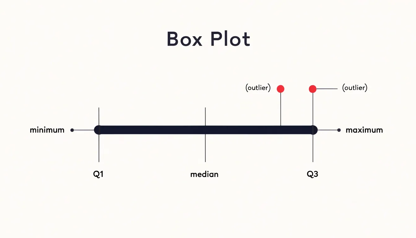
- Minimum: The lowest typical observation, marked by the end of the lower whisker.
- First quartile (Q1): The bottom edge of the box.
- Median: A line drawn inside the box showing the central value and hinting at any skew.
- Third quartile (Q3): The top edge of the box. Together, Q1 to Q3 span the interquartile range (IQR), containing the middle 50% of all observations.
- Maximum: The highest typical observation, marked by the end of the upper whisker.
Box plots are particularly useful for spotting outliers. Values that fall more than 1.5 times the interquartile range beyond either edge of the box are plotted as individual points, drawing immediate attention to extreme observations.
They also excel at side-by-side comparison. Placing several boxes along a shared axis lets viewers contrast the variance, median, and range of multiple datasets in a single view. Tightly clustered boxes signal low variability, while elongated boxes and long whiskers reveal a broader spread. This makes box plots a staple of exploratory analysis and quality control, where the shape and dispersion of data matter as much as the average.
Heat Maps
Heat maps represent numerical values as a spectrum of colors within a two-dimensional matrix. Each cell corresponds to a combination of two variables—such as hours of the day and days of the week—while the cell’s color encodes the magnitude of a third variable, like website traffic or sales volume. Warmer colors (reds, oranges) typically indicate higher values, while cooler colors (blues, greens) denote lower values, allowing viewers to spot patterns, density, and anomalies that would be hard to see in a table of raw numbers.
Common applications include:
- Spatial density: In store layouts, heat maps show which aisles attract the most foot traffic; in geographic data, they illustrate concentrations like population density or crime rates across regions.
- User behavior: Overlays on website screenshots, generated from clickstream or scroll data, glow in warm colors where users click or linger, helping designers optimize layouts.
- Correlation grids: A heat map of a correlation matrix uses one hue for strong positive correlations and a contrasting hue for strong negative ones, summarizing relationships across many variable pairs at once.
Treemap
A treemap displays hierarchical data as a set of nested rectangles that fill a single rectangular frame. Each top-level category occupies a large parent rectangle that encloses smaller rectangles for its subcategories, continuing down through as many levels as the data requires. The area of each rectangle is proportional to its quantitative value, so a category twice as large as its sibling occupies twice the area.
Containment shows how smaller parts roll up into larger wholes, while color typically provides a second channel of meaning—distinguishing top-level branches, encoding an additional variable like growth rate, or grouping related items. Labels and borders help users navigate deeper levels, though very small rectangles may need to be aggregated or left unlabeled due to space constraints.
Treemaps handle large trees containing hundreds or thousands of items, such as budget allocations across departments and programs, file storage broken down by folder, or market share segmented by sector and company. Compared with a bar chart, a treemap adds hierarchical structure; compared with a node-link diagram, it adds proportional weight, showing both the shape of a hierarchy and the size of its parts in one frame.
Waterfall Charts
Waterfall charts show how a starting value turns into a final value through a sequence of positive and negative adjustments. The chart begins with a full bar representing the initial balance. Subsequent bars float between the previous running total and the new total: positive adjustments extend upward and negative adjustments extend downward in a staircase pattern, usually colored differently to distinguish gains from losses. Connector lines between bars trace the running total until a final full bar summarizes the ending balance.
This step-by-step structure is widely used in finance to break down changes in net income, cash flow, or budget variances. For example, a waterfall chart can start with gross revenue and show each expense category as a downward step to arrive at net profit, making it clear which factors drive the final result.
Sankey Diagrams
Sankey diagrams map the flow of energy, materials, financial resources, or other quantities through a system. Their defining feature is that the width of each band is proportional to the quantity it carries, so viewers can read relative magnitudes directly from the diagram.
Flows generally move from left to right: inputs enter on one side, split or merge across intermediate nodes (such as conversion, storage, or distribution stages), and exit on the other side as useful output or waste. Because every branch is drawn to scale, system efficiency is immediately visible. A thick band might show a power plant’s total fuel input, while narrower branches show shares diverted to losses or byproducts; the ratio of useful to wasted streams reveals where intervention would yield the greatest savings.
Sankey diagrams can display dozens of interconnected flows across multiple nodes, making them well suited to supply chains, national energy budgets, industrial material cycles, and organizational budgets. Color coding can distinguish flow categories without disturbing the proportional reading of widths.
Choropleth Maps
Choropleth maps shade predefined geographic regions—such as countries, states, counties, or census tracts—according to a statistical value for each area, such as population density, median income, voter turnout, or disease prevalence. Darker or more saturated shades typically represent higher values and lighter shades represent lower values, turning regional tables into spatial patterns of clusters, gradients, and outliers.
Two structural limitations require care:
- Uniformity within boundaries: Filling an area with a single shade treats the entire region as uniform, masking internal variation.
- Area bias: Geographically large regions draw more visual attention than small ones, which can make a sparse rural district look more prominent than a dense urban one.
Designers mitigate these issues by choosing appropriate geographic units, setting sensible class intervals, and matching the color palette to the data structure. A sequential palette (running from pale to deep) suits data that moves in one direction from low to high. A diverging palette (two contrasting hues meeting at a neutral midpoint) suits data centered on a reference value such as zero, an average, or a target.
Funnel Charts
Funnel charts track a sequential, multi-stage process using horizontal bars whose widths correspond to the number of records or participants remaining at each step. The chart begins with the widest bar at the top—such as total site visitors, leads, applicants, or cart initiations—and narrows at each subsequent stage as participants drop off, ending with the narrowest bar for completed purchases, enrollments, or closed cases.
The taper of the funnel shows conversion efficiency at a glance. A gentle taper means steady progression, while a sharp contraction pinpoints a stage with high friction—whether caused by a confusing form, a slow approval step, an unexpected cost, or a manual handoff. Analysts typically annotate the bars with both stage-to-stage conversion rates and the cumulative rate from entry to completion. Because the stages are ordered and aligned, teams can easily compare funnels across time periods, channels, or customer segments to see whether changes at a bottleneck stage widen the bars below it.
Candlestick Charts
Candlestick charts show price action across trading sessions (such as a minute, hour, day, or week) by encoding four values for each period: open, high, low, and close (OHLC).
- The body: Formed by the range between the opening and closing prices. A long body indicates strong directional movement; a short body suggests indecision between buyers and sellers.
- The color: A green or white body typically means the price closed above the open (buyers dominated), while a red or black body means it closed below the open (sellers dominated).
- The wicks (or shadows): Thin lines extending above and below the body to mark the session’s highest and lowest prices. Long wicks signal volatility and price rejection, where traders pushed the price to an extreme before it retreated prior to the close.
Traders read combinations of bodies and wicks across multiple candles to gauge market sentiment, trends, support and resistance levels, and periods of consolidation. For example, a series of long green bodies with short wicks points to strong bullish momentum, while a doji—a candle where the open and close are nearly equal—reflects equilibrium and potential hesitation or reversal.
Frequently Asked Questions
What are bar charts best used for?
Bar charts compare discrete categories using rectangular bars whose lengths encode values. They work well for ranked lists, survey responses, or datasets where long category labels need room, especially with horizontal bars.
How do line graphs show trends over time?
Line graphs track trends over continuous periods by connecting data points to form a continuous path. They are well suited to time-series data where the sequence of observations matters.
What does a pie chart show?
A pie chart represents a whole divided into slices, where each slice’s central angle and area correspond to its share of the total. It is suited to static part-to-whole compositions such as budget allocations or market share breakdowns.
What is a histogram used for?
A histogram shows the distribution of a continuous numerical variable by sorting observations into equal-width intervals called bins. The height of each bar reflects the count or proportion of observations in that interval.
How can you tell positive and negative correlation on a scatter plot?
On a scatter plot, positive correlation appears as points trending upward from left to right, while negative correlation slopes downward. A narrow band of points suggests a strong association, and a wide, diffuse spread suggests a weak one.
How does a box and whisker plot show outliers?
A box plot marks values that fall more than 1.5 times the interquartile range beyond either edge of the box as individual points. This draws immediate attention to extreme observations.
Tony Astor
Tony writes about data visualization and the tools people use to build charts and dashboards. More about Data Illustrator