Treemap: How to Show Hierarchical Part-to-Whole Data
 By Tony Astor ·

Treemap
A treemap displays a hierarchy as nested rectangles, where each rectangle’s area is proportional to a quantitative value attached to a category or subcategory. The largest rectangle represents the whole, partitioned among child categories by their measured values, then subdivided recursively. The layout tiles space without gaps or overlaps, making treemaps useful for comparing part-to-whole relationships across many categories.
Table of Contents
Treemap
A treemap displays a hierarchy as a single rectangle subdivided into smaller rectangles, where each rectangle’s area corresponds to a quantitative value attached to a category or subcategory. The largest rectangle represents the whole, and its area is partitioned among child categories in proportion to their measured values. Each child is then subdivided in the same way for its own subcategories, producing a nested structure of rectangles within rectangles. Viewers can compare magnitudes across the full hierarchy at a glance, from the largest top-level category down to the smallest leaf node.
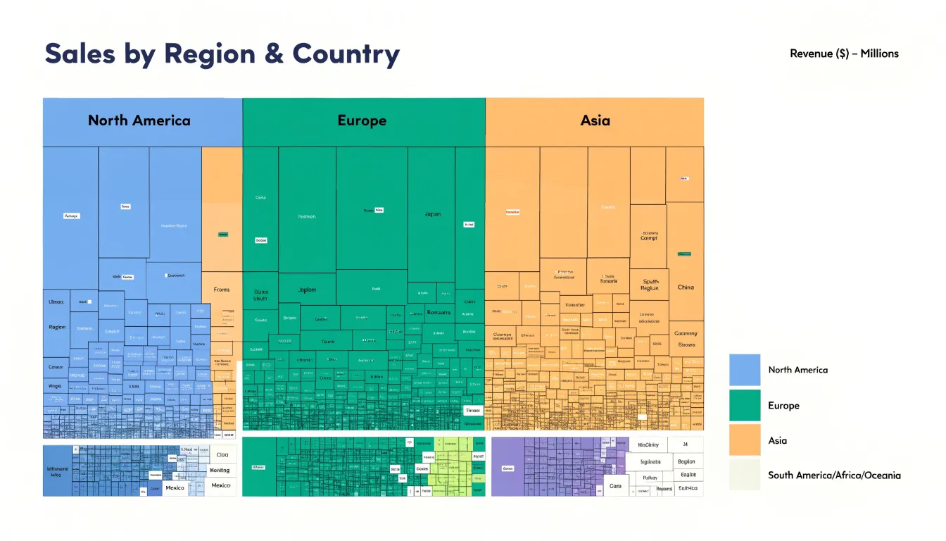
The layout algorithm arranges rectangles to tile the available space without gaps or overlaps, filling a constrained visual frame completely. This makes treemaps especially useful when screen space is limited, since every pixel carries data rather than being wasted on whitespace or axes. Aspect ratios matter considerably in practice: elongated slivers are harder to compare and label than squarish shapes, so layout methods such as slice-and-dice, squarified, and strip arrangements trade off between strict proportionality and readability.
Color and labeling add a second and third dimension of information. Color often indicates a separate attribute such as category membership, growth rate, or performance against a target, while labels identify categories directly within their rectangles when space allows. Nesting depth is visible through borders and containment, allowing a viewer to trace from an outer category inward to its constituents.
The result is a compact, hierarchical overview suited to large numbers of categories, where relative size is the primary question and precise value lookup can be handled through interactive tooltips or drill-down.
Hierarchical Data
Hierarchical data organizes information into levels, where each parent category contains one or more child categories nested beneath it. At the top sits a single root node representing the whole dataset, which branches into major categories, subcategories, and finally the most granular leaf elements. A typical example is a sales dataset split by region, then country, then product line, with individual records forming the leaves of the tree. Every node except the root has exactly one parent, capturing both membership and containment: a child belongs to its parent, and the parent’s total encompasses the sum of its children.
Treemaps translate this structure into space by placing child rectangles physically inside their parent’s boundary. Because children divide the parent’s area among themselves based on a chosen measure like revenue or file size, proportional relationships between levels remain intact.
Moving from the root to a leaf takes the viewer through successive levels of containment, each enclosed by the previous. Because the layout is generated recursively, treemaps scale to deep hierarchies without losing the parent-child relationships that give the data its meaning. Viewers can see both the overall distribution across top-level categories and the internal composition of each category within a single view.
Part-to-Whole
Treemaps excel at revealing part-to-whole relationships across many categories at once, and comparing them with pie and stacked bar charts clarifies when each format serves best. Pie charts work well for a small number of slices, typically five or fewer, because the human eye struggles to compare wedge angles accurately beyond that point. Stacked bar charts handle more categories along a single axis, yet as segments multiply, each one narrows until differences in length become hard to judge. Treemaps sidestep this problem by allocating area recursively, so even dozens of categories remain visible and comparable through both area and position.
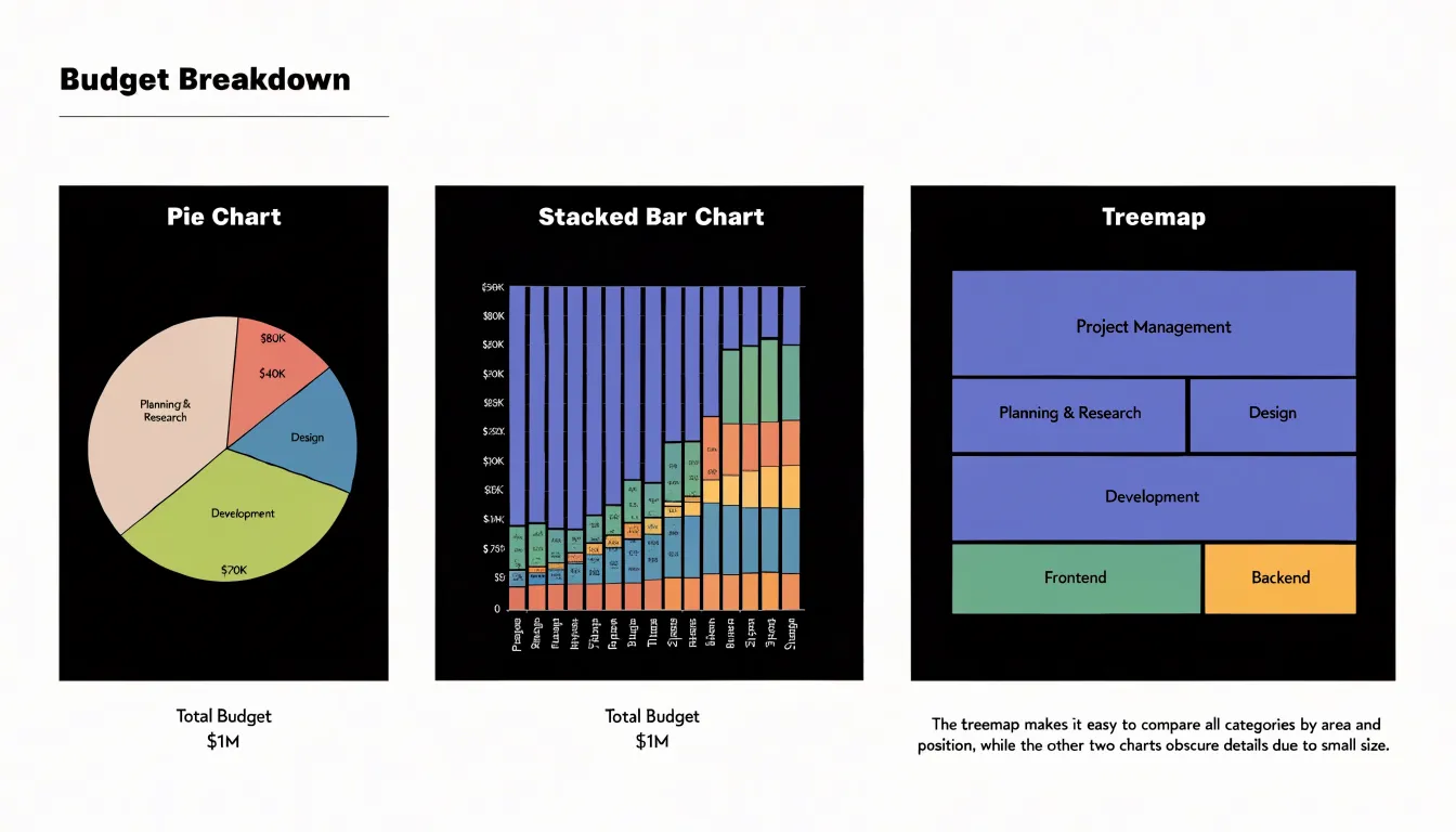
When a dataset contains a large number of categorical breakdowns, treemaps preserve detail that pie charts and stacked bars would compress into unreadable slivers. Hierarchical structure is another decisive factor: treemaps natively represent nested groupings, such as product categories within regions within quarters, while pie and stacked bar charts flatten hierarchy into a single level or require multiple separate charts.
Choosing between these formats depends on the analytical question:
- Pie chart: Intuitive for a quick impression of a simple split.
- Stacked bar chart: Offers clean alignment for comparing segments across a shared baseline.
- Treemap: Provides the clearest overview of relative size when the breakdown is complex, hierarchical, or extensive, supporting rapid scanning of dominant and minor contributors alike.
Anatomy
The visual anatomy of a treemap rests on three core encoding elements: rectangle size, color, and labels.
Rectangle size is governed by an area scale, where a rectangle twice as large as another encodes a value twice as great. Because human area perception is less precise than length perception, treemaps work best for relative comparisons rather than exact readings.
Color serves as a second encoding channel to represent a categorical variable or a secondary quantitative measure. Sequential or diverging palettes can highlight patterns across the hierarchy, with darker shades indicating higher values or different categories.
Labels provide the textual context that makes the treemap interpretable, typically displaying the category name and sometimes the value inside the rectangle. Ensuring legibility requires contrasting text colors and adjusting font sizes based on rectangle dimensions. For small rectangles where text does not fit, labels may be truncated, omitted, or attached via leader lines.
Data Prep
Data prep for treemap software begins with organizing source material into a clean, flat table where every row represents one node in the hierarchy.
- Assign unique identifiers: List each entity (such as a department, product line, or folder) and assign every row a unique integer or short code in a dedicated ID column.
- Establish parent references: Add a parent ID column recording the identifier of the row’s immediate superior. Top-level nodes, which have no parent, should receive a consistent placeholder such as a blank cell or a fixed null value like zero. Keeping parent references separate from display names makes the structure unambiguous for software to parse.
- Attach quantitative values: Place the metric that determines rectangle area in its own column, using a consistent unit free of symbols, commas, or text. Rows that serve only as containers (aggregating their children) should either carry a zero or be omitted from the value column according to the tool’s convention. Verify that every parent ID matches an existing ID and that no node points to itself, since orphaned rows will be dropped or misdrawn.
- Add labels and clean the table: Label each row with a human-readable name and, where useful, a descriptive column for notes or categories. Keep column headers short and standardized, remove merged cells and totals rows, and confirm there are no gaps in key fields. A quick sort by parent ID reveals the hierarchy’s shape, and a spot check of sibling sums against parent totals catches errors early before mapping the fields in software.
Sizing
Achieving a reliable correspondence between a raw metric and the geometric dimensions of each rectangle requires a deliberate scaling step.
The process begins by choosing a scale. Values may be mapped linearly, or through a square-root transformation applied to the side lengths, which yields the same proportional result once the sides are multiplied. Square-root scaling is common in practice because it lets an algorithm work in one dimension at a time while still producing correct two-dimensional areas. Normalization then converts the full range of data values into a fixed total area—typically the available canvas—so the sum of all tile areas matches the display region regardless of the absolute magnitude of the numbers.
Once the total area is fixed, layout algorithms allocate space recursively, preserving the ratio between sibling areas at every level. Residual rounding from pixel constraints is usually absorbed by adjusting the last tile in a row or by carrying fractional remainders forward, keeping aggregate error small.
Small values can fall below the threshold of visibility, so very low metrics may be aggregated or given a minimum size, a decision that should be documented.
Color
While rectangle area communicates the primary metric, hue or saturation can encode a secondary metric such as sentiment, growth rate, or variance.
For categorical data like sentiment, map each class to a distinct hue drawn from a qualitative palette, keeping saturation and lightness consistent so differences in tone are read as category distinctions rather than magnitude.
For continuous data, use a sequential or diverging scale:
- Diverging scales suit metrics with a meaningful midpoint, such as zero percent growth, using one hue for positive values, another for negative values, and a neutral tone at the center. Saturation can encode intensity while hue carries direction, letting viewers spot strong movers.
- Sequential scales suit variance or change scores without a natural pivot point.
Keep the primary area metric visually dominant so secondary color choices do not overwhelm size comparisons. Limit palettes to a handful of steps, maintain adequate contrast against labels and borders, and include a legend that names both variables and states their units. Test the result by checking whether someone can rank rectangles by size without distraction from the color, and read the color pattern independently.
Layout
The central goal of any treemap layout algorithm is to keep each rectangle as close to square as possible, since long, thin slivers make labels hard to fit and areas difficult to compare.
The squarified layout algorithm addresses this by arranging sibling rectangles in rows or columns and switching orientation whenever doing so keeps the worst aspect ratio under control. The algorithm sorts items by size from largest to smallest, then greedily adds items to the current row as long as the resulting aspect ratios stay within an acceptable threshold. When adding another item would worsen the aspect ratio, the algorithm finalizes the current row and begins a new one along the remaining edge of the parent rectangle, keeping width-to-height ratios close to one.
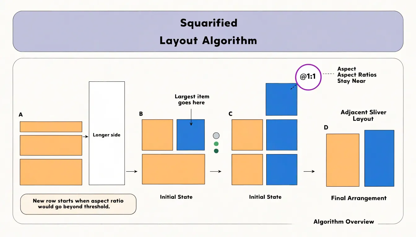
Several practical refinements improve this approach:
- Order input data by descending value: Large items anchor each row while small items fill the remaining space.
- Set a sensible aspect ratio threshold: A value around 2.5 to 4 balances compactness against computational cost.
- Apply scaled padding: Adding a few pixels between rectangles helps distinguish adjacent items, and scaling that padding with hierarchy depth keeps parent-child relationships visually apparent.
- Test against real datasets: Real-world edge cases, such as many near-equal values or a single dominant value, reveal awkward geometry that idealized test data might miss.
Nesting
When a dataset contains three or more nested hierarchical levels, additional rectangles, labels, and color variations can overwhelm the reader. Several strategies manage this complexity:
- Limit visible depth: Restrict the initial view to two or three levels of nesting, using filtering or drill-downs to explore deeper structures.
- Group minor items: Aggregate small or less important subcategories into an “Other” group to reduce the number of visible tiles.
- Use nested padding and shading: Inset each level within its parent (“nesting with padding”) or use borders and shading to delineate groups. Subcategories can also inherit a lighter or darker shade of the top-level parent’s color.
- Maintain consistent ordering: Sort rectangles within each group by size or alphabetical order to help users navigate.
Interactivity
Interactivity transforms a treemap from a static overview into a dynamic exploration tool by offloading detail from the main canvas.
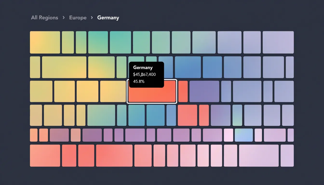
- Tooltips: Hovering over a rectangle displays precise values, full labels, and context that would clutter the static view.
- Hover states: Highlighting the hovered rectangle while dimming others provides visual feedback, helping users isolate and compare specific elements.
- Drill-down and breadcrumbs: Clicking a rectangle can reveal the next level of the hierarchy, such as individual products within a department. Breadcrumbs or back buttons maintain context as users navigate deeper into areas of interest and return to the high-level overview.
Design
Three core design rules keep a treemap readable as data density increases:
- Structural whitespace: Deliberate gaps between tiles and groups act as breathing room for the eye. Consistent spacing and padding around parent groups prevent the chart from collapsing into an undifferentiated mosaic, giving each block a clear boundary without requiring heavy outlines.
- Clear color contrast: Neighboring tiles need enough separation in luminance and hue to remain distinct even at small sizes, and sequential scales should progress intuitively from low to high. Muted borders or thin strokes can reinforce separation without competing with fill colors so any two touching tiles can be told apart at a glance.
- Selective labeling: Reserve direct labels for tiles with enough area to hold text comfortably, anchoring the reader’s orientation on major categories while leaving minor blocks unlabeled to preserve legibility across the chart.
Pitfalls
Even well-constructed treemaps can falter due to common implementation pitfalls:
- Truncated labels: Forcing long text into small tile boundaries cuts off category names. Use ellipses, abbreviations, external leader lines, or dynamic hover labels instead.
- Tiny, unclickable tiles: In dense treemaps, small rectangles are difficult to interact with, especially on touch devices. Fix this by aggregating small values into an “Other” category, enforcing a minimum tile size in the layout algorithm, or providing zoom and keyboard navigation.
- Misleading color scales: Using a sequential scale for categorical data implies order where none exists, while rainbow scales create false visual boundaries. Scaling color by area instead of the secondary value also distorts perception. Match the palette to the data type and maintain consistent color mapping across all treemaps in a dashboard.
Use Cases
Treemaps are widely used for budgets and storage breakdowns, where quantities at every hierarchical level need to be compared simultaneously.
Government spending: A national, municipal, or regional budget can be shown as a single rectangle subdivided by ministry or department, then into programs and line items. Viewers instantly see that major areas like health and defense occupy large shares of the total while smaller agencies appear as narrow slivers, with color encoding year-over-year spending changes.
Corporate budgets: Mapping divisions at the top level, departments beneath them, and individual cost centers at the leaves lets executives identify major cost drivers and spot categories that are disproportionately large relative to their function. Even budgets with hundreds of line items fit on a single screen, supporting faster comparisons than long tables of figures.
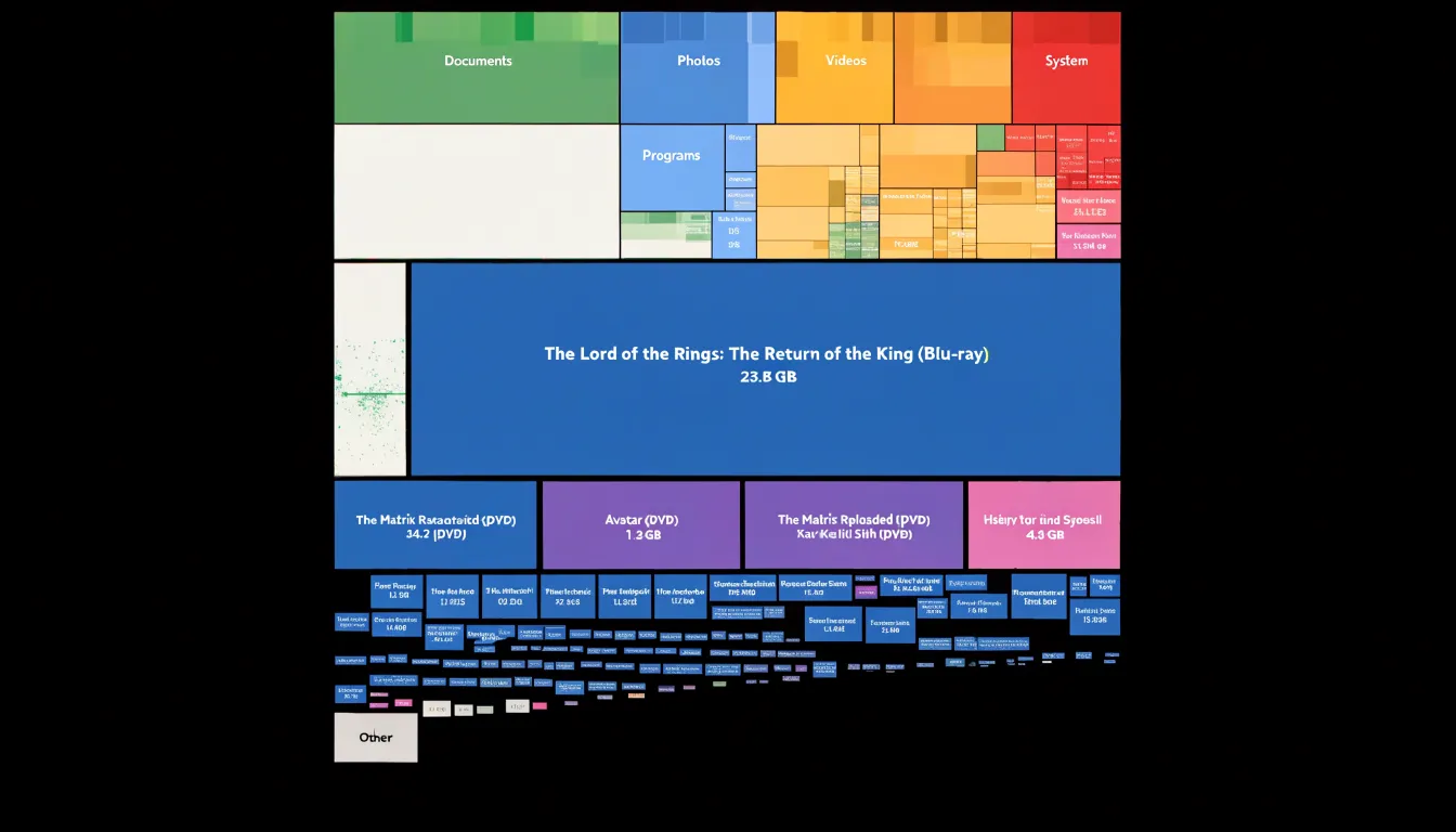
Digital storage: Disk-space analyzers visualize a hard drive with folders as nested rectangles and files sized proportionally to their byte count. System administrators managing servers and ordinary users cleaning up personal machines can immediately locate the handful of folders or media files consuming most of the capacity without clicking through directory trees one level at a time.
Tools
Creating a treemap depends on the data size, update frequency, and required customization of your working environment:
- Excel: Includes a built-in treemap in its standard chart gallery. Users select hierarchical data in two columns, insert the chart, and adjust labels, colors, and levels through the formatting pane. It suits small datasets and quick reporting, though customization is limited.
- Tableau: Treats treemaps as a native mark type. Analysts drag a dimension onto the marks card, size rectangles by a measure, and layer color encodings, filters, and interactive tooltips.
- Power BI: Offers a built-in treemap visual that supports live data refreshes and customization via the marketplace and JSON-based theme files.
- D3.js: Provides low-level JavaScript primitives, including a treemap layout function that computes rectangle positions from nested data. It enables fine-grained control over transitions, labels, and interaction at the cost of more setup work.
- Python (Plotly Express and Squarify): Plotly Express includes a treemap function that accepts a dataframe with path columns and outputs interactive HTML charts. For static rendering, libraries like Squarify compute rectangle coordinates for Matplotlib.
Dashboard
A treemap earns its place in an executive dashboard when it answers a question that trend lines and single-number KPI tiles cannot: where, within a total, is the weight concentrated?
Give the treemap roughly a quarter to a third of the dashboard’s horizontal space, placing it in the middle or lower tier of the grid beside the trend charts rather than beneath the headline KPIs. This leaves the top band for headline metrics while keeping the treemap large enough for legible labels. If a dashboard already carries several charts, the treemap should serve as the single composition view, replacing a pie or crowded bar chart.
Sizing should follow data density: a dozen top-level categories with shallow nesting fit in a compact panel, whereas deeper hierarchies require more room or interactive expansion. To balance visual weight, use muted palettes and thin borders so the treemap does not pull attention away from the KPI band, reserving saturated color for the specific segment under discussion. Connecting the treemap to interactive dashboard filters allows it to respond to selections made in other charts, functioning as a supporting lens on the data.
Frequently Asked Questions
What is a treemap used for?
A treemap displays a hierarchy as rectangles whose areas correspond to quantitative values, allowing viewers to compare magnitudes across the full hierarchy at a glance. It is especially useful for a compact, hierarchical overview of large numbers of categories where relative size is the primary question.
When should I use a treemap instead of a pie chart or stacked bar chart?
Pie charts work well for a small number of slices, typically five or fewer, while stacked bar charts handle more categories but become harder to judge as segments narrow. A treemap provides the clearest overview of relative size when the breakdown is complex, hierarchical, or extensive.
How should I prepare hierarchical data for a treemap?
Start with a clean, flat table where every row represents one node, with unique identifiers, parent references, and the quantitative value that determines rectangle area in its own column. Top-level nodes should receive a consistent placeholder for parent ID, and the table should be cleaned by removing merged cells and totals rows and checking that parent IDs match existing IDs.
How can I keep labels readable in a treemap?
Labels identify categories directly within their rectangles when space allows, and legibility requires contrasting text colors and adjusting font sizes based on rectangle dimensions. For small rectangles where text does not fit, labels may be truncated, omitted, or attached via leader lines, and direct labels should be reserved for tiles with enough area to hold text comfortably.
What is the squarified layout algorithm in a treemap?
The squarified layout arranges sibling rectangles in rows or columns and switches orientation whenever doing so keeps the worst aspect ratio under control. It sorts items by size from largest to smallest, then greedily adds items to the current row as long as the resulting aspect ratios stay within an acceptable threshold.
How can I manage a treemap with three or more nested levels?
Limit the initial view to two or three levels of nesting, using filtering or drill-downs to explore deeper structures. You can also aggregate small or less important subcategories into an “Other” group, use nested padding and shading, and maintain consistent ordering within each group.
Tony Astor
Tony writes about data visualization and the tools people use to build charts and dashboards. More about Data Illustrator