Tidy Data: How to Structure Data for Charting
 By Tony Astor ·

Tidy Data
Tidy data is a standardized table structure in which each variable forms a column, each observation forms a row, and each observational unit forms a table. This layout gives plotting and statistical tools a predictable structure, making data easy to reshape, validate, and visualize without custom cleaning.
Table of Contents
- Tidy Data Basics
- Variables and Observations
- Columns and Rows
- Cells and Values
- Spotting Messy Data
- Reshaping Data
- Cleaning Column Names
- Handling Missing Values
- Standardizing Units
- Splitting and Combining Columns
- Fixing Date Formats
- Preparing Categorical Data
- Checking Data Types
- Exporting to Charting Tools
- Final Checks and Dashboard Overview
Tidy Data Basics
Tidy data provides a consistent, predictable structure that graph software depends on to render accurate visuals. When each variable forms a column, each observation forms a row, and each type of observational unit forms a table, the data becomes immediately usable by plotting libraries and statistical tools. This structure eliminates ambiguity: the software knows exactly where to find the values for the x-axis, the y-axis, and any grouping or faceting variables. As a result, the mapping from data to visual elements is direct and reliable, reducing the risk of misplotted points, swapped axes, or missing categories.
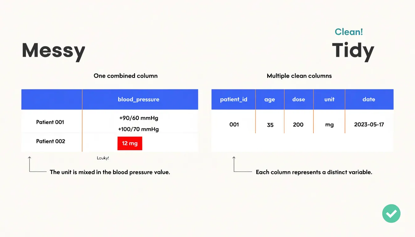
Clean formatting also ensures that data types are interpreted accurately. In tidy data, a date column contains only dates in a standard format, a numeric column contains only numbers, and a categorical column contains only consistent labels. This uniformity allows graphing software to apply the appropriate scales, transformations, and statistical summaries without manual intervention.
Moreover, tidy data supports reproducibility and automation. Once data is in a tidy format, the same code can be reused across different datasets or updated versions because the structure remains consistent. This is particularly valuable when creating multiple charts or dashboards, as plotting commands can be written generically and applied repeatedly. The alternative—messy data with values embedded in column headers or multiple variables crammed into one column—requires custom cleaning and reshaping for each new visualization, which is time-consuming and error-prone.
Variables and Observations
Every dataset rests on two fundamental concepts: variables and observations. A variable is a measured attribute—the property or characteristic that describes something of interest, such as height, temperature, revenue, or treatment group. An observation is a single unit that carries those measurements, such as one person, one day, one transaction, or one experimental subject. Getting these definitions right at the design stage is the cheapest way to ensure a dataset behaves predictably under analysis.
Identifying variables means deciding what is being measured and at what level of granularity. A dataset of patient visits has a variable for age and a variable for blood pressure, and each row captures one visit. When the boundary between variables becomes blurred, structural flaws emerge. A column labeled ‘blood pressure before and after treatment’ secretly contains two variables compressed into one cell, forcing future readers to parse text before they can compute anything. A column that mixes patient age with measurement units, such as ‘45 years,’ similarly buries a variable inside formatting, pushing cleanup work downstream.
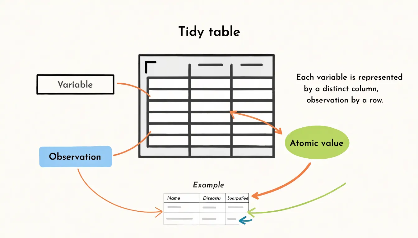
Identifying observations means deciding what one row represents. A dataset might contain one row per customer, one row per order, or one row per order line, and each choice yields a different structure. Trouble begins when a single table mixes levels, so some rows describe customers while others describe orders. Aggregations then become ambiguous, and row counts no longer map cleanly onto counts of anything meaningful. Clear definitions let analysts compare rows, group columns, and validate completeness without guesswork.
Columns and Rows
In a tidy table, columns separate what was measured, while rows separate whom or what it was measured on.
Each column carries a single variable. Age forms one column, income forms another, and date of visit forms a third. Every cell beneath a column header holds a value of that same kind, measured in the same units and drawn from the same domain. A reader scanning down a column encounters comparable pieces of information, which makes sorting, filtering, and summarizing straightforward. This arrangement allows the analyst to reason about a variable as a coherent whole, computing its distribution or checking its range of values without disentangling mixed content.
Each row corresponds to one observation—a single complete record of a person, transaction, sensor reading, or clinical trial. All measurements belonging to that unit sit together on the same line, capturing a snapshot of the entity at a given moment or condition. When new information arrives about a case, it joins the existing row rather than being scattered elsewhere. This horizontal cohesion means that comparing observations involves comparing rows, and adding a new case means appending a row without disturbing the surrounding structure.
Statistical functions, plotting libraries, database queries, and machine learning pipelines all expect to find variables in fields and observations in records. This rule converts messy, human-oriented spreadsheets into a predictable substrate for reproducible analysis.
Cells and Values
A data cell should hold one atomic value: a single number, a single category, or a single date. This gives each column a consistent type—numeric, categorical, or temporal—so a plotting library can read it as a continuous axis or a set of categories without preprocessing. Grouping, sorting, and aggregating all behave predictably when values are atomic. Selecting all rows where dose exceeds 10 becomes a simple numeric comparison rather than a string search.
Concatenated text breaks this at the point of use. When a cell contains ‘12 mg’ or ‘patient 47, male, 62 years’, the column no longer has a consistent type, and every downstream operation must parse free text before it can do anything useful. A column of strings like ‘12 mg’, ‘8 mg’, ‘15 mg’ looks tidy at a glance, but the numbers inside are locked away. To plot dose against response, you must first split the text and convert the numeric part, and that parsing step is where errors creep in: inconsistent units, stray spaces, and missing separators.
The same problem appears with combined identifiers or packed demographic fields, where several facts share a single cell. Separating those facts into their own columns keeps each value addressable, so filtering on sex, sorting by age, or plotting dose all draw from clean, typed data without string operations. The cost of splitting is paid once at tidying time; the benefit accrues every time the data is queried.
Spotting Messy Data
Before building any chart, open the raw dataset and scan the first several rows for structural flaws that distort visual outputs:
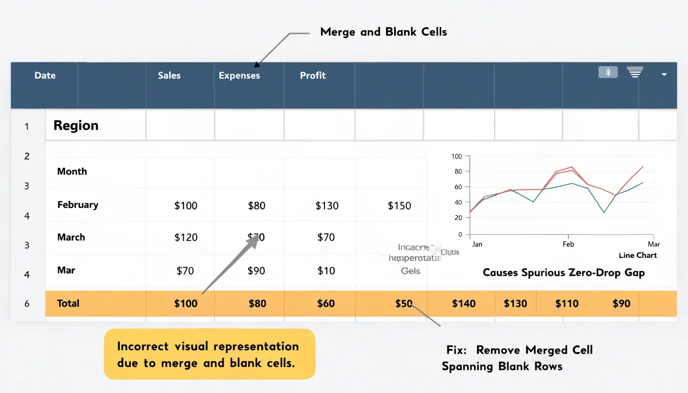
- Unformatted headers: Headers typed by hand often include trailing spaces, inconsistent capitalization, line breaks inside a cell, or dual-row titles where one row holds a category and the next holds units. These irregularities cause plotting tools to treat a header as a data series, inserting a stray line or bar that distorts the scale. Check that every column header sits in a single row, occupies one cell, and uses a consistent naming pattern.
- Merged cells: When a spreadsheet merges a cell across several columns or rows to create a visual grouping, the underlying data often shifts. Import tools may read the merged value once and leave neighboring cells empty, producing gaps that a chart renders as zero or missing values. Merging rows to label repeated categories is especially risky, because the empty cells below the merge can break grouping logic in pivot tables and charts. Look for centered text spanning multiple columns and blank cells beneath a category label.
- Embedded summary rows: Totals, subtotals, averages, or notes placed inside the data region get read as ordinary observations. A chart then plots a total alongside its components, inflating the axis and misleading the reader. Scan for rows containing words like total, subtotal, average, or grand total, and for rows where values clearly exceed the surrounding figures. Move these summaries to a separate sheet or exclude them from the chart range.
Reshaping Data
Reshaping data between wide and long representations is a frequent preparatory step, and the decision of when to pivot depends on the graphing engine you intend to use.
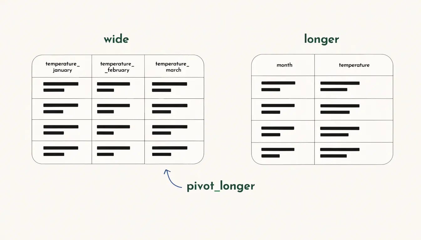
A wide dataset stores each variable in its own column, with one row per observational unit, so temperature readings for January, February, and March each occupy a separate column. A long dataset collapses those repeated measurement columns into a pair of key and value columns, producing one row per observation and recording the variable name alongside its value.
Graphing engines differ in which shape they accept as input:
- Long data: Many plotting libraries, including ggplot2 and its grammar-of-graphics relatives, expect long data because they map a grouping variable to an aesthetic such as color or panel. This requires that all measurements live in a single column with an accompanying label. Passing wide data to such an engine forces awkward workarounds or produces a single combined series instead of separate lines or facets.
- Wide data: Spreadsheet charts and some statistical modeling functions expect wide data where each series appears as its own column.
Inspect the plotting function’s documentation before reshaping. If the engine asks for an x column, a y column, and a grouping column, pivot longer first. If it asks for one column per series, pivot wider. Reshaping is cheap and reversible, so converting early and experimenting with the engine often clarifies the requirement faster than reading specifications. Keep the original data intact and store the reshaped version in a separate object so you can pivot back when a downstream step demands the opposite shape.
Cleaning Column Names
Raw datasets often have column headers with spaces, mixed capitalization, punctuation, and special characters such as parentheses, slashes, or percent signs. While readable in a spreadsheet, these headers create friction in code because many plotting libraries and query languages treat spaces and special characters as operators or delimiters, causing a header like “Sales (Q1)” to break a pipeline.
Rename headers once at the start as part of a documented cleaning step. A good convention keeps each name in lowercase, replaces spaces with underscores, and strips out symbols that require awkward quoting. Names like “Total Revenue ($)” become total_revenue, and ”% Change 2023” becomes pct_change_2023.
Make each column name a short, meaningful identifier that anyone reading the script can understand without consulting documentation. Prefer full words over cryptic abbreviations, and be consistent: if one column uses total_revenue, the related column should be total_cost rather than TotalCost or total cost. Consistency lets you reference columns with predictable patterns, reduces typos, and makes collaboration easier.
Handling Missing Values
How you handle missing values has a direct effect on the accuracy of any trendline you draw. The first step is to understand why a cell is blank. A missing measurement may reflect a sensor failure, a skipped survey question, or a value that does not apply to that record. Recognizing the mechanism behind the gap helps you choose an approach that preserves the meaning of the data:
- Imputation: Fill blanks with a sensible estimate, such as the column mean or median, a value carried forward from the previous observation, or a prediction from a regression model built on related columns. Imputation keeps your dataset at full size and maintains continuity in time series, though it introduces assumptions that should be documented.
- Deletion: Dropping rows with missing entries is simple and defensible when gaps are few and occur at random, but removing too many rows can bias a dataset and thin out the observations a trendline depends on.
- Explicit labeling: Mark missing entries with a clear placeholder or a separate indicator column rather than silently erasing them. This keeps the absence visible and lets downstream analysis treat it deliberately.
Whichever route you take, prevent blanks from being silently converted into zeros or distorting summaries. Recording your chosen method alongside the dataset, and noting how many values were affected, gives readers confidence in the resulting trendlines.
Standardizing Units
When a dataset contains measurements recorded in different units—such as currencies from multiple countries, weights in pounds and kilograms, or temperatures in Celsius and Fahrenheit—failing to convert them to a common scale leads to misleading charts.
Each unit carries its own magnitude, and mixing them on the same axis distorts the visual representation. If a chart plots revenue where some entries are in US dollars and others in euros without conversion, the axis scale becomes meaningless. A value of 1000 euros might appear equal to or larger than 1000 dollars, even though their actual magnitudes differ. The visual distance between points no longer reflects true differences in the data, causing viewers to draw incorrect conclusions about trends, comparisons, or outliers.
Converting all measurements to a single unit—through exchange rates, conversion factors, or simple arithmetic—ensures that every number on the axis shares the same reference frame. Perform unit conversion early, before aggregation or plotting, to avoid compounding errors. Standardization also simplifies axis labeling and interpretation, as viewers do not need to mentally adjust for varying units.
Splitting and Combining Columns
Composite fields often arrive as a single text column holding several data points fused by a delimiter, such as a full address packed with street, city, and postal code, or a product label combining category and size. Parsing these fields into discrete variables begins with identifying the delimiter and confirming it appears consistently across every row. String splitting functions then divide each value at the delimiter and assign the resulting segments to new columns. Watch for edge cases: missing delimiters, inconsistent spacing, and values that themselves contain the delimiter all require a cleaning pass before parsing, since a single stray comma can shift every downstream segment into the wrong column.
Combining works in the opposite direction, joining complementary categories into a single field where that union serves the analysis. When a chart legend carries dozens of near-duplicate entries, merging related levels into broader groups produces a legend readers can scan at a glance. Concatenation joins two columns with a separator, useful for building a unique identifier or a human-readable label such as a region paired with a year. Categorical mapping offers a softer form of combination, assigning many detailed categories to fewer summary groups while preserving the original values in a separate column for reference.
Document each transformation, along with the rules used to merge or split values, so colleagues can trace how the tidy table was derived from its raw source.
Fixing Date Formats
A single dataset might contain “January 3, 2024,” “03/01/2024,” “2024-01-03,” and “3 Jan 24” all referring to the same day, drawn from different source systems or manual entry. A computer sorting these strings alphabetically produces nonsense: values starting with a letter cluster together, values beginning with numbers sort by their first digit, and the chronology collapses. When such strings feed a time-series graph, the x-axis ordering becomes arbitrary and lines zigzag.
The remedy is to convert every date value into the ISO 8601 format: YYYY-MM-DD. In this layout, the year comes first, followed by the month and the day, each padded to a fixed width. Because the most significant component is first, ordinary lexicographic string sorting coincides with chronological sorting. The string “2023-11-02” sorts before “2024-01-03” because the leading digits compare correctly, requiring no special date parser to establish order.
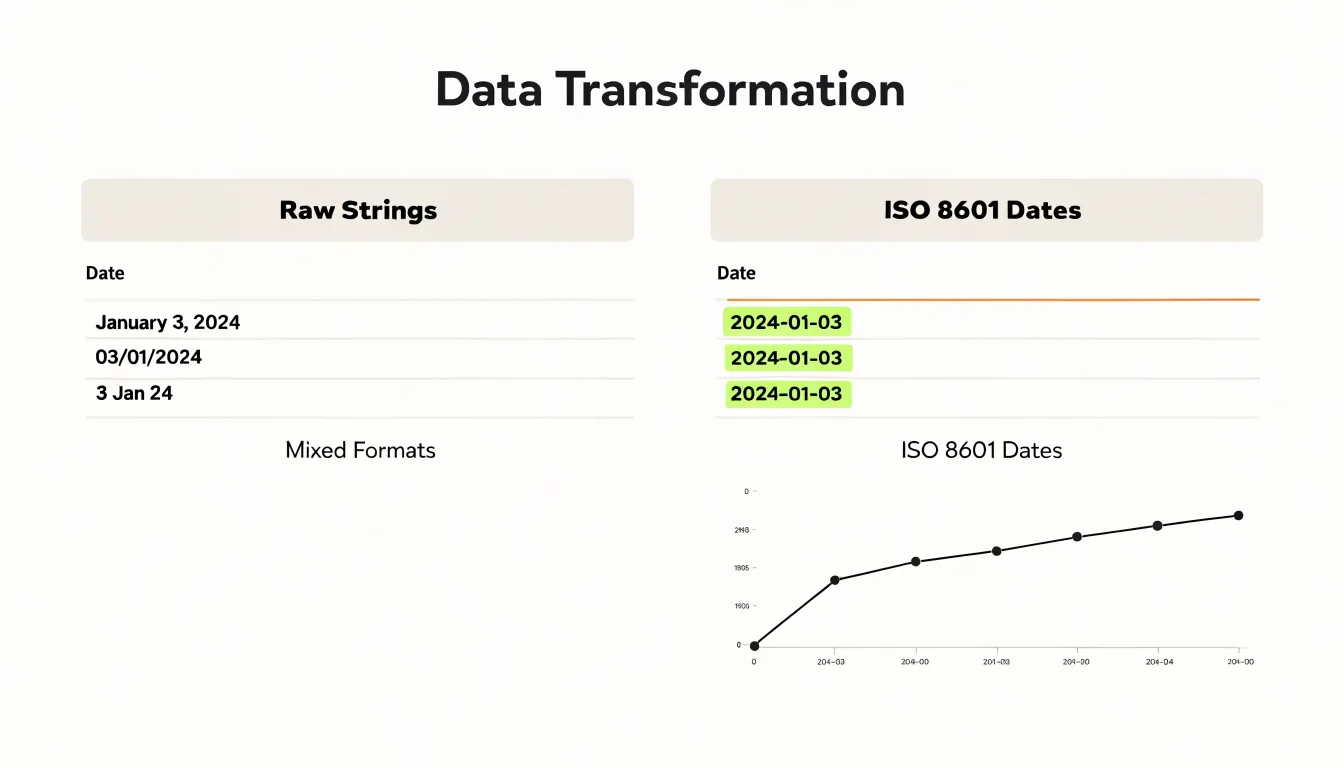
Applying this conversion consistently guarantees that monthly rollups align to the right periods, rolling averages follow the true sequence of observations, and graphs display a continuous, monotonic time axis. It also makes validation easier: any value that fails to parse as ISO signals a genuine data quality problem rather than a stylistic variation.
Preparing Categorical Data
Survey responses, exported spreadsheets, and hand-entered records often contain the same category recorded in several ways, producing cluttered bar charts with near-duplicate labels that fragment counts.
Consolidating redundant category names is the first step toward legible visuals. For example, ‘New York’, ‘NY’, and ‘new york’ may all refer to the same place, while ‘Large’, ‘L’, and ‘lg’ describe one size. Before plotting, review the unique values in each categorical column and map synonyms and abbreviations onto a single canonical name using a lookup table.
Standardizing text casing and spacing supports the same goal:
- Casing: Inconsistent capitalization creates visual noise on axis labels and splits categories that computers treat as distinct strings. Apply a uniform convention, such as title case for proper nouns or lowercase for generic labels, using a string function.
- Whitespace: Trim leading and trailing whitespace, since a stray space produces a category that looks identical to its neighbor but sorts and groups separately.
Together, these steps reduce the number of unique categories, shorten labels so they fit along the axis, and ensure each bar represents the full count for its category.
Checking Data Types
Numeric fields stored as text cause silent failures when you attempt to chart or aggregate. Instead of summing revenue values to a total, charting software may concatenate them, count them as distinct categories, or refuse to place them on a continuous axis.
To detect mistyped numbers, inspect how your tool reports the field type and sort the column. Numeric values sorted as text order themselves lexically, so “10” appears before “9” and “100” before “20”. Other reliable signals include values that refuse to right-align in a spreadsheet, cells carrying a leading apostrophe, warning triangles or text icons beside the column header, and summary functions that return counts instead of sums.
Once detected, correction depends on the tool:
- In a spreadsheet: Re-type the cell, use a value conversion function, or clear the apostrophe prefix to coerce the string to a number.
- In code: Strip thousands separators, currency symbols, and stray whitespace first, since these characters force the field to remain text. Then cast the column explicitly and verify the cast succeeded by checking for nulls or error values introduced during conversion.
After conversion, re-sort the column to confirm numeric ordering and run a quick sum or mean to verify the values behave as numbers.
Exporting to Charting Tools
When exporting a tidy dataset to a dedicated charting tool such as Tableau, Excel, or Power BI, the file formatting determines how smoothly the import behaves:
- Structure: A clean CSV or JSON file starts with one header row, one observation per row, and one variable per column, with no merged cells, blank separator rows, or decorative titles above the data. Because import wizards detect types from the first rows they encounter, keeping the top of the file free of notes prevents columns from being misread as text. For JSON exports, a flat array of objects with identical keys imports reliably, whereas deeply nested structures may require flattening first.
- Encoding and delimiters: Save files as UTF-8 to preserve accented characters and non-Latin scripts, which older encodings can turn into garbled symbols. For CSVs, make delimiter and quoting rules explicit, and quote any field containing commas, line breaks, or quotation marks so the parser does not split a single value across columns.
- Formats and missing values: Use ISO 8601 dates (such as
2024-03-15) and keep numeric columns free of embedded units, currency symbols, or thousands separators, which belong in the chart application’s presentation layer. Represent missing values consistently, either as empty fields or as a single agreed code, so the tool can distinguish absence from zero.
Keep a copy of the original data in its source format so any transformation applied for visualization can be traced and reproduced.
Final Checks and Dashboard Overview
Before a dataset and its visuals leave your hands, run through a structured audit:
- Check row and column counts: Compare totals against the source extract to confirm the number of records matches expectations for the reporting period. A sudden jump or drop in row count is often the first sign of a broken join or a duplicated import.
- Review column types and ranges: Confirm that numeric fields contain only numbers, dates parse correctly, and categorical values stay within their known set. Scan for blanks and placeholders that slipped through cleaning, and check the minimum and maximum of every measure against plausible bounds—a temperature column that maxes out at 999 or a sales figure below zero deserves a second look.
- Verify uniqueness and key integrity: Confirm that identifier columns contain no duplicates where uniqueness is required, and that every foreign key resolves to a valid parent record. Spot-check a handful of rows end to end, tracing a value from the raw source through your transformation steps to the final table.
- Audit visual accuracy: Open every chart in the dashboard and confirm that axis scales, units, and labels match the underlying columns. Cross-check a few plotted values against the tidy table directly. Confirm that filters and date ranges update all connected visuals consistently, and that totals shown on summary cards agree with the sums in the dataset.
- Document the audit: Record the audit date, the checks performed, and any exceptions noted to give reviewers context and make future refreshes easier to validate.
Frequently Asked Questions
What is tidy data and why does it matter for graphing?
Tidy data provides a consistent, predictable structure where each variable forms a column, each observation forms a row, and each type of observational unit forms a table. This structure helps graphing software find the values for the x-axis, y-axis, and grouping or faceting variables, reducing the risk of misplotted points, swapped axes, or missing categories.
What is the difference between a variable and an observation in a dataset?
A variable is a measured attribute, such as height, temperature, revenue, or treatment group. An observation is a single unit that carries those measurements, such as one person, one day, one transaction, or one experimental subject.
Why should each data cell contain only one atomic value?
A cell should hold a single number, category, or date so each column has a consistent type and plotting, grouping, sorting, and aggregating behave predictably. When a cell contains concatenated text like “12 mg,” the numbers are locked inside strings and must be parsed before use, which is where errors can creep in.
What common signs of messy data should I look for before building a chart?
Before charting, scan the raw dataset for unformatted headers, merged cells, and embedded summary rows. These flaws can cause plotting tools to treat a header as a data series, render gaps as zero or missing values, or plot totals alongside components and distort the axis.
How do I know whether to reshape data wide or long for a charting tool?
Inspect the plotting function’s documentation before reshaping. If the engine asks for an x column, a y column, and a grouping column, pivot longer first; if it asks for one column per series, pivot wider.
How should missing values be handled before drawing a trendline?
First understand why a cell is blank, since the gap may reflect a sensor failure, a skipped survey question, or a value that does not apply. Then choose imputation, deletion, or explicit labeling, and prevent blanks from being silently converted into zeros or distorting summaries.
Tony Astor
Tony writes about data visualization and the tools people use to build charts and dashboards. More about Data Illustrator