Strip Plot: Showing Every Data Point in a Distribution
 By Tony Astor ·

Strip Plot
A strip plot is a graph that displays every individual data point as a separate mark along a single axis, preserving the full distribution, clusters, gaps, and outliers that summary statistics like means can hide. Small horizontal jitter separates overlapping points, and transparency reveals density. It suits small to moderate samples and complements box plots and bar charts.
Table of Contents
Strip Plot
Every dataset carries information in its individual observations, and those observations frequently differ from one another in ways that summary statistics cannot express. A strip plot places each data point as a discrete mark along a single axis, so the viewer sees the full distribution of values as they actually occurred. This approach preserves granular detail that aggregated measures erase. A mean and a standard deviation can describe a symmetric, well-behaved distribution accurately, yet the same two numbers can arise from wildly different underlying shapes. When individual points are shown, clusters, gaps, and outliers remain visible, and the reader can judge the spread and density directly rather than inferring them from a compressed summary.
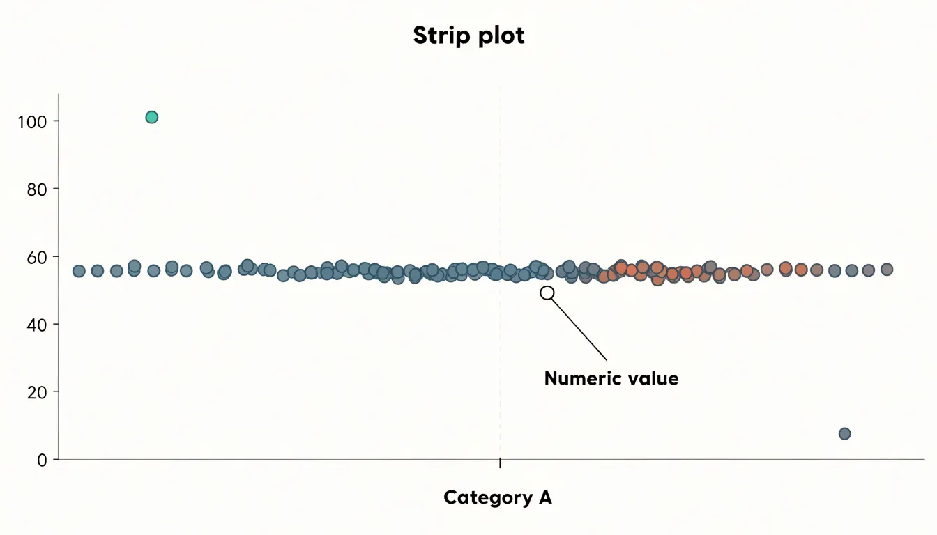
Masking is a common hazard in visualization. Overplotting occurs when multiple observations share the same value and collapse into a single visible position, hiding the true count. Grouped bars or box plots can obscure bimodal distributions, where two distinct clusters sit at opposite ends of a range and the average falls in a sparse middle region that contains almost no real observations. A strip plot exposes these features because each observation occupies its own mark. Small horizontal jitter can be applied to separate coincident points, so repeated values appear as vertical density rather than a single dot, revealing where the data concentrate.
Showing raw points also supports verification. A reader can trace any summary claim back to the observations that produced it, which builds trust in the analysis and invites scrutiny of unusual cases. Outliers appear as they are rather than being smoothed away by an averaging process. For small and moderate sample sizes, the strip plot is especially effective because the individual marks remain distinguishable and the overall shape of the data is legible at a glance. The result is a transparent view of the data that respects its complexity and gives the audience the evidence needed to draw their own conclusions about pattern, spread, and anomaly.
Strip Plot vs Bar Chart
A bar chart is often the first tool reached for when summarizing data across categories, with each bar representing a mean or total. This familiar format communicates a single number per group, which makes comparison easy at a glance. The trouble is that a mean is an abstraction that collapses every observation into one point. Two groups can share an identical average while containing completely different internal structures, and a bar chart gives no hint of that difference.
In a bimodal dataset, the average can fall in the empty gap between two extreme clusters, describing a value that no actual observation holds. A skewed distribution presents a similar problem, since the mean gets pulled toward the long tail and may sit far from where most data points actually lie. Outliers compound the issue by dragging the average away from the bulk of the observations. In each case the bar stands tall and confident, while the underlying distribution remains invisible.
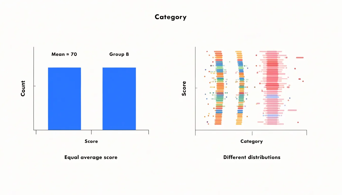
A strip plot addresses this directly by plotting every observation along the category axis. A bimodal group shows two distinct bands of points, while a skewed group reveals a dense concentration on one side trailing off into scattered points on the other. Outliers appear as isolated marks rather than silently distorting a summary. Reading a strip plot alongside a summary value gives the mean its proper context, showing whether it represents the data well or masks an important pattern. For exploratory analysis, this transparency makes strip plots a valuable complement to conventional bar charts.
Strip Plot
Because every observation occupies its own position on the axis, extreme values stand out plainly. An unusually high or low measurement appears as a lone mark separated from the main cluster, drawing the eye without any need for calculation. In aggregated views, that same extreme value would be folded into an average and hidden. The strip plot keeps it visible, so a single anomalous reading in a clinical trial, a manufacturing batch, or a sensor log announces itself immediately and invites closer inspection.
The display also conveys spread in a direct, visual way. The distance between the smallest and largest marks shows the full range at a glance, while the density of marks along the axis reveals where most observations concentrate. Gradual transitions become apparent as patterns in the distribution of points, letting a viewer see at once whether values are tightly grouped around a central region or spread broadly across the axis, and whether the distribution is symmetric or skewed.
Multiple observations at the same value can be offset slightly to show their number, so ties remain visible. Subgroups can be distinguished by position or color, allowing comparisons of spread between categories within the same frame. The result is a compact picture in which outliers and overall variance are both immediately legible before any modeling or aggregation takes place.
Strip Plot
When dozens of points occupy identical or nearly identical coordinates along the categorical axis, the plot hides the true distribution: a cluster of twenty overlapping dots looks identical to a single dot. Two complementary techniques help recover this lost information.
The first is jitter, which adds a small amount of random noise to the position of each point along the categorical axis, spreading coincident markers into a visible cloud whose width reflects local density. The amount of jitter should be tuned carefully; too little leaves points stacked, while too much distorts the perceived category boundaries and can make adjacent groups bleed into each other. Seeding the random number generator keeps results reproducible across runs.
The second technique is transparency, implemented through the alpha channel. By rendering each marker semi-transparent, areas where many points overlap accumulate pigment and appear darker, while sparse regions remain faint. This turns overplotting into a visual density cue, letting readers estimate how many observations lie beneath any given marker. Alpha values in the range of 0.2 to 0.5 often work well for moderately sized datasets, and a slight edge stroke can help individual points remain legible when alpha is low.
Combining jitter with transparency is especially effective: jitter separates points that would otherwise coincide exactly, and alpha encodes the residual overlap that jitter cannot resolve. Together these adjustments show both the full spread of the data and the concentration of observations within dense regions.
Strip Plot With Box Plot
Overlaying a strip plot onto a box plot brings together two complementary views of a dataset in a single graphic. The box plot supplies the summary statistics: the median line marks the center of the distribution, the box edges show the first and third quartiles, and the whiskers extend toward the range of typical values. These elements give a quick sense of central tendency, spread, and skew. The strip plot adds the individual observations along the same axis, jittered slightly on the categorical axis so that overlapping values remain visible. Viewers can read the summary metrics and inspect the raw data at the same time.
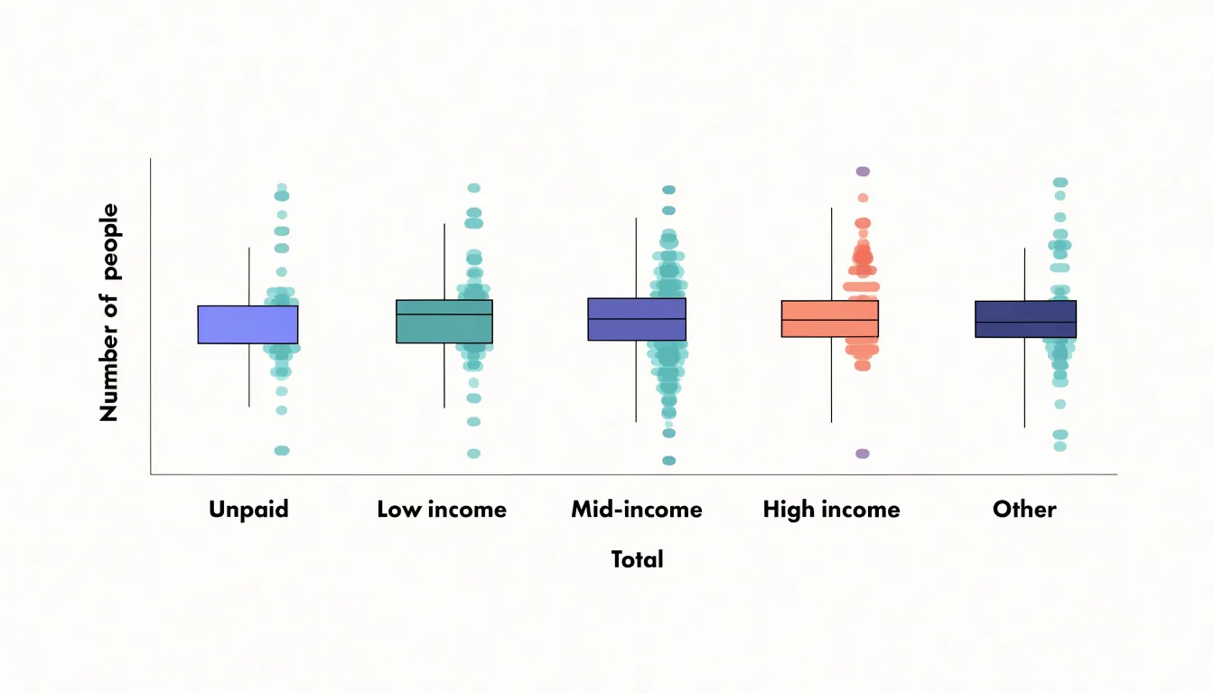
This pairing is useful because a box plot of a small sample may suggest a clean distribution, while the overlaid points reveal gaps, clusters, or a handful of distant values that the quartiles compress. Conversely, the box plot anchors the cloud of points, making it easier to see where the mass of observations sits relative to the median and how far the extremes stretch beyond the whiskers.
When building the combined plot, follow these steps:
- Draw the box plot first with a neutral fill.
- Place the strip points on top using a contrasting color, partial transparency, and a small horizontal offset.
- Choose a jitter width so points spread enough to avoid stacking without suggesting precision that the data lacks.
- Keep the axis shared so both layers refer to the same scale.
- With larger samples, reduce point size or increase transparency to prevent the strip layer from obscuring the box.
The combined figure works well for comparing several groups side by side, since each category shows its summary metrics and its full set of observations together.
Grouped Strip Plot
A grouped strip plot arranges individual data points along a categorical axis while splitting each category into sub-groups that sit side by side. The primary categorical variable defines the main positions along the horizontal axis, and a secondary grouping variable subdivides each position into adjacent columns. Within every column, each observation is drawn at its measured value on the vertical axis with a small amount of horizontal jitter.
Structuring the plot this way supports direct visual comparison across multiple groups. Placing sub-groups adjacent within the same category keeps the comparison local, so the eye can move from one column to the next without traversing the whole figure. Readers can compare medians by noting where points concentrate, assess spread by observing how far markers extend above and below the center, and spot skew or multimodality from the shape of the point cloud. Consistent marker size, color, and jitter width across all columns keep these judgments fair and reduce the risk of misreading one group against another.
Practical construction involves several choices:
- Assign a distinct color or shape to each sub-group to make the grouping legible at a glance, and include a legend to clarify the mapping.
- Order the sub-groups consistently across every category to prevent confusion when scanning the chart.
- When sample sizes differ substantially between sub-groups, vary the jitter or note counts in axis labels to keep the comparison honest.
Strip Plot
Transparency becomes especially valuable when sample sizes are small. With only a handful of data points, conventional summary statistics can paint a distorted picture. A mean calculated from five or ten values can be pulled sharply by a single outlier, and a standard deviation computed on such a thin base offers little reassurance about spread. A strip plot sidesteps these problems by letting the reader see the full set of values without any aggregation standing between them and the raw data.
When working with small samples, the shape of a distribution is often irregular in ways that summary numbers conceal. Two groups might share nearly identical means and variances while one contains a tight cluster of values and the other is scattered with gaps. Showing every point makes it easier to judge whether a reported average actually represents the typical case or sits in an empty region between clusters.
The technique also supports honest uncertainty. With few observations, any inference about a population rests on shaky ground, and a plot that shows every point communicates this fragility directly. Readers can count the values, notice a lone extreme observation, and understand that a single data point carries substantial weight. For small datasets, strip plots function as a compact and faithful record of the evidence itself, allowing analysts and audiences to reason from the actual observations.
Strip Plot
As sample sizes grow, a strip plot accumulates marks until individual observations begin to merge into an undifferentiated band. The threshold at which this happens is not a fixed number; it depends on the plotting area, the marker size, and the degree of overlap among categories. A few hundred points spread across a wide chart may still read clearly, while the same count compressed into a narrow axis turns into a solid smear. Readers can no longer distinguish individual observations, trace gaps, or judge local density by eye. The plot has crossed from informative to merely decorative.
Detecting this threshold involves attention to a few practical signals:
- Markers routinely sit on top of one another.
- The visual mass of a category stops changing as points are added.
- Jitter must be increased so much that the horizontal positions become meaningless.
Setting marker opacity can buy some headroom, but transparency has limits once the underlying points are dense enough to saturate the color. At that point, alternative visualizations serve the reader better:
- Violin plot: Summarizes the full shape of the distribution, showing where values cluster and how the density tapers, while consuming a single column of space per category.
- Histogram (or side-by-side histograms): Makes the count in each bin explicit and keeps comparisons between groups straightforward.
- Box plot: Offers a compact summary of median, spread, and outliers, scaling gracefully to large samples.
The choice should follow the analytical question. If exact values and ordering matter, keep the strip plot and reduce the data through sampling or binning. If the shape of the distribution is the point, a violin plot or histogram will convey it far more legibly than a dense cloud of overlapping markers.
Strip Plot
When a dataset contains meaningful subgroups within its main categories, color becomes a powerful tool for making those subgroups legible. By mapping a categorical variable to hue, each subgroup receives its own distinct color. Analysts can see at a glance whether a particular subgroup clusters at the high or low end of the distribution, whether its values spread widely or concentrate tightly, and whether subgroups overlap heavily or separate cleanly.
This kind of hue mapping is especially useful when the number of subgroups is modest, since a small palette of clearly distinguishable colors keeps the plot readable without overwhelming the viewer. Color also reduces visual confusion in dense regions where points pile up, because the eye can follow the trajectory of a single color through the mass of dots.
Practical implementation involves choosing a palette with sufficient contrast, ordering the colors consistently across panels, and pairing color with a clear legend or direct labels. When subgroups are nested within broader categories, hue can be layered alongside position or faceting to reinforce the hierarchy of information, turning a simple one-dimensional display into a richer visual summary.
Strip Plot
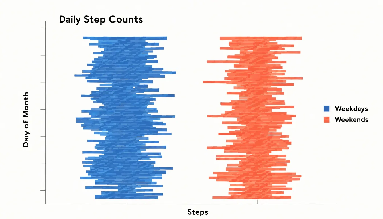
Daily health tracking generates a steady stream of individual measurements, and strip plots give those measurements a clear visual home. A person who wears a fitness tracker accumulates one step count per day, one resting heart rate reading per morning, and one sleep duration per night. Plotted as a strip plot, each day becomes a single mark positioned along a horizontal axis according to its value, with the days stacked in a light vertical scatter so that overlapping values remain visible. Over a month or a season, this arrangement reveals the spread of activity levels at a glance: clusters of similar step counts, isolated high days from a weekend hike, and low days during illness or travel all appear as distinct features of the distribution.
Heart rate variation benefits from the same treatment. Resting heart rate readings collected each morning form a natural one-dimensional series, and a strip plot shows whether the values bunch tightly around a baseline or fan out during periods of stress, poor sleep, or increased training load. Because each point corresponds to a specific day, the plot preserves the individuality of every reading. Adding a second strip plot beneath the first—one for steps and one for heart rate—lets a reader compare the two distributions directly and notice whether low-activity days coincide with elevated heart rate readings.
Strip plots also work well for comparing groups of days. Separating weekday logs from weekend logs into parallel strips makes differences in typical step counts immediately visible without requiring a summary table. The same approach applies to before-and-after periods, such as the weeks following a new exercise routine. For personal health tracking, where sample sizes are small and every measurement matters, the strip plot keeps individual daily records in view while communicating the overall pattern.
Strip Plot in Python
Seaborn provides a straightforward path to building strip plots in Python through the sns.stripplot() function. A typical workflow begins by importing the necessary libraries, loading a built-in dataset such as tips or penguins, and passing the categorical variable to the x argument and the numeric variable to the y argument. This minimal call produces a vertical arrangement of points grouped by category.
From that starting point, several parameters control the plot’s behavior and appearance:
jitter: By default, Seaborn applies a small amount of jitter along the categorical axis. SettingjittertoTrue,False, or a numeric value gives direct control over the horizontal spread. A value like0.25often works well for datasets with moderate density, while disabling jitter entirely helps when precise positional accuracy matters more than visibility.hueanddodge: Thehueparameter colors points according to a second categorical variable to compare subgroups within each category. Combininghuewith thedodgeparameter (or with split settings in related functions) separates overlapping categories into side-by-side columns.- Custom styling: Parameters such as
palettefor color selection,sizefor marker dimensions,markerfor point shape,alphafor transparency, andlinewidthfor edge definition help tailor the chart to a specific report. order: Controls the sequence of categories along the axis.
You can also layer sns.stripplot() over a box or violin plot to pair raw observations with summary statistics. Combining these parameters in a single call makes sns.stripplot() a flexible tool for both exploratory analysis and polished presentation.
Strip Plot in R
In R, the ggplot2 package provides an expressive grammar for building strip plots using two core geometries: geom_point() and geom_jitter(). Starting with geom_point() gives a straightforward one-to-one mapping of each observation to a plotted location. To prevent identical values from overlapping along a single categorical position, geom_jitter() adds a small random displacement to each point. The jitter is controlled through the width and height arguments, which tune how far points spread along each axis; keeping height small preserves categorical alignment while width reveals clustering. Setting a seed in R ensures this random displacement is reproducible when figures are regenerated for a final manuscript.
Aesthetic mapping inside aes() lets you map color, shape, or size to a grouping variable, such as coloring points by treatment or assigning shapes to sites. Fine-tuning then moves to the scale, position, and theme layers:
- Scales and themes:
scale_color_manual()orscale_shape_manual()let you pick palettes and symbols suited to print or screen, whilethemeadjustments control axis labels, panel backgrounds, and legend placement. - Position adjustments:
position_jitterdodge()combines jittering with dodging, so grouped points sit side by side rather than piling up. - Summary overlays: Adding a summary statistic, such as a mean or median marker via
stat_summary(), gives context to the spread of individual points.
Together, these layers produce publication-ready strip plots within a reproducible R workflow.
Strip Plot vs Swarm Plot
In a strip plot, the only thing separating points within a category is random jitter applied along the perpendicular axis. Each point receives its offset independently, drawn from a random distribution such as a uniform or normal spread centered on the category line. This independence gives the strip plot its characteristic look: a loose, textured band of dots. Because each offset is random, two points with nearly identical values can still land in the same place, producing overplotting in dense regions. Increasing the jitter width reduces collisions, but at the cost of exaggerating the horizontal footprint of the category and blurring its clean alignment. Because there is no coordination between points, the method cannot guarantee that any two markers stay apart.
A swarm plot takes an algorithmic rather than random approach. Points are placed sequentially along the category axis in order of their values, and each new point is shifted away from the center line only as far as needed to avoid touching the markers already positioned. The displacement follows a deterministic rule that checks nearby points and pushes the newcomer outward, often using a fixed marker radius to define the exclusion zone. The result is a symmetric, hive-like arrangement in which no markers overlap and the silhouette of the swarm traces the shape of the data distribution. The width of the swarm at any vertical position directly indicates local density, making the visual envelope an informative feature rather than a byproduct of randomness.
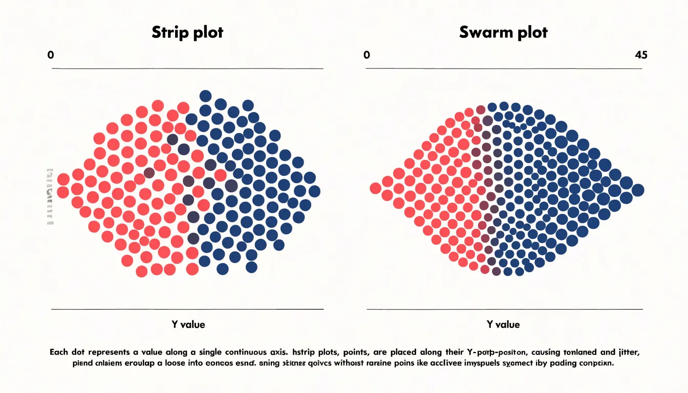
The trade-off is computational and structural. Swarm placement requires sorting and collision checks, so it scales less gracefully than simple jittering, and the resulting arrangement can look more rigid than a strip plot. Both methods reveal individual observations that a box or violin plot would hide, differing only in whether that revelation comes through scattered texture or orderly, collision-free packing.
Strip Plot Design
Thoughtful visual design ensures a strip plot remains easy to scan, honest about its data, and accessible to the widest possible audience:
- Point markers: Markers should be large enough to register clearly at the intended viewing size, yet small enough that overlapping points remain distinguishable. Use semi-transparent fills to reveal density and a thin contrasting outline to keep individual marks legible against busy backgrounds. Where categories matter, pair color with shape so that readers who cannot distinguish hues can still follow the groupings.
- Axis scaling: The continuous scale should start and end at values that frame the data without exaggeration. Maintain consistent scales across panels to allow direct comparison, and use clearly labeled tick marks at sensible intervals. When many categories are present, give the category axis enough room for readable labels and consider ordering categories by median or count to make patterns apparent.
- Gridlines and borders: Light, thin gridlines behind the points support the reading of values without competing with the data. Remove heavy borders around the plotting area and other unnecessary chart junk to keep attention on the distribution.
- Typography and accessibility: Choose a clean sans-serif typeface at a size that remains readable on small screens, with axis titles that explain units and category meanings. Ensure sufficient contrast between text and background, and never rely on color alone to convey information. Include alt text and concise captions to extend the chart’s reach to readers using assistive technology.
Strip Plot Dashboard
Integrating strip plots into reporting dashboards requires intentional layout and consistent styling so they complement surrounding metrics without cluttering the view. Strip plots work especially well alongside summary tables or KPI cards, providing the granular detail and outlier visibility behind aggregated numbers.
To build an effective strip plot dashboard, apply these guidelines:
- Placement and layout: Place strip plots in side-by-side panels where users can compare distributions across groups. Maintain uniform axis scales and visual styling across all panels to facilitate fair comparison.
- Managing complexity: Avoid overcrowding by limiting the number of strip plots per dashboard. Use interactive filtering or faceting to handle large numbers of categories, and keep the visual design minimal.
- Interactivity: Add interactive features like tooltips or brushing to let users inspect individual records and explore patterns across linked charts, ensuring these features support rather than distract from the core message.
- Responsiveness and documentation: Ensure the plots render legibly across different screen sizes. Finally, document your design choices—such as whether points are jittered or what summary lines represent—to help users interpret the distributions accurately.
Frequently Asked Questions
What does a strip plot show that summary statistics do not?
A strip plot places each observation as a discrete mark along a single axis, so you can see clusters, gaps, outliers, spread, and density directly. This preserves granular detail that aggregated measures may erase.
Can a strip plot be used instead of a bar chart?
A strip plot can complement a bar chart by showing every observation behind a category, including bimodal groups, skew, and outliers that a mean bar may hide. A bar chart still communicates a single summary number per group for easy comparison.
How do you prevent overlapping points in a strip plot?
Use small horizontal jitter to separate coincident points and semi-transparent markers so overlapping areas appear darker. Tune jitter carefully, because too much can distort perceived category boundaries and make adjacent groups bleed into each other.
How do you overlay a strip plot on a box plot?
Draw the box plot first with a neutral fill, then place jittered strip points on top using a contrasting color, partial transparency, and a small horizontal offset. Keep the axis shared, and with larger samples reduce point size or increase transparency so the strip layer does not obscure the box.
What should you use instead of a strip plot for large sample sizes?
When points merge into an undifferentiated band, alternatives include a violin plot, a histogram or side-by-side histograms, and a box plot. The article notes that the threshold depends on plotting area, marker size, and overlap, not a fixed number.
How do you create a strip plot in Python?
Use Seaborn’s sns.stripplot() function, passing the categorical variable to x and the numeric variable to y. Parameters such as jitter, hue, dodge, palette, size, alpha, and order control the plot’s appearance and grouping.
Tony Astor
Tony writes about data visualization and the tools people use to build charts and dashboards. More about Data Illustrator