Stream Graph: What It Is and When It Works
 By Tony Astor ·
Stream Graph
A stream graph is a variation of a stacked area chart that displays changes in category volume over time as an organic, flowing shape. Each category forms a layer stacked vertically along a continuous time axis, with its thickness representing value at that moment, centered around a horizontal baseline.
Table of Contents
Stream Graph
A stream graph is a variation of a stacked area chart that shows changes in category volume over time through an organic, flowing shape. Each category is represented as a layer stacked vertically along a continuous time axis, with its vertical thickness corresponding to the category’s value at that point in time.
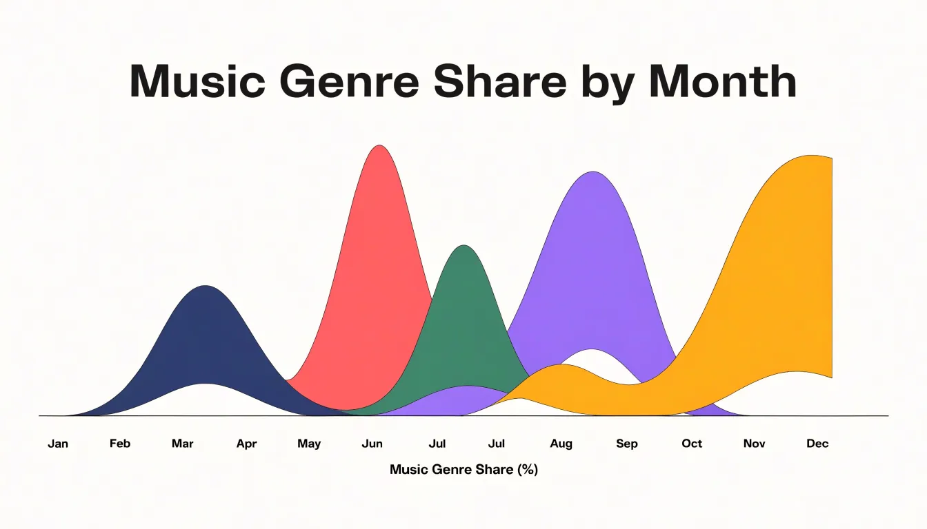
The overall graph is centered around a horizontal baseline, which can be straight or curved, with layers arranged symmetrically above and below it. This symmetry, combined with smooth interpolation between data points, minimizes abrupt changes in thickness and creates an undulating appearance. Because the stacking order of categories is typically fixed, viewers can track individual layers across time to spot trends, seasonal patterns, and sudden shifts in composition.
Stream Graph
Reading a stream graph begins with the horizontal axis, which encodes time from left to right. The spacing between gridlines or tick marks shows the duration each segment represents. Because uneven intervals can distort perception, check whether the axis is scaled linearly and whether data points are evenly sampled. The horizontal extent also helps you judge whether trends near the edges are meaningful or simply artifacts of where the dataset begins and ends.
Vertical thickness carries each category’s magnitude at a given moment. Because bands stack around a central baseline, a band’s vertical position reflects both its own size and the sizes of the bands beneath or above it. Compare thicknesses at the same horizontal position to see relative proportions, and watch how a band swells or narrows across time to detect growth or decline. Sudden vertical jumps often signal shifts in category composition rather than changes in total volume.
Color provides category identity and metric attributes. Distinct hues separate series, while varying saturation or lightness within a hue can indicate subcategories or secondary measures. Consistent hue assignments across related charts support comparison. When colors blend or change mid-band, inspect the underlying data for reclassification or merging.
Stream Graph
Because the bands are continuous rather than rigid bars, the eye reads the chart as a moving system. A sudden surge appears as a bulge that pushes neighboring bands aside and reshapes the chart’s contour. A sharp decline narrows or pinches off into a thin ribbon, leaving a visible gap where volume once was.
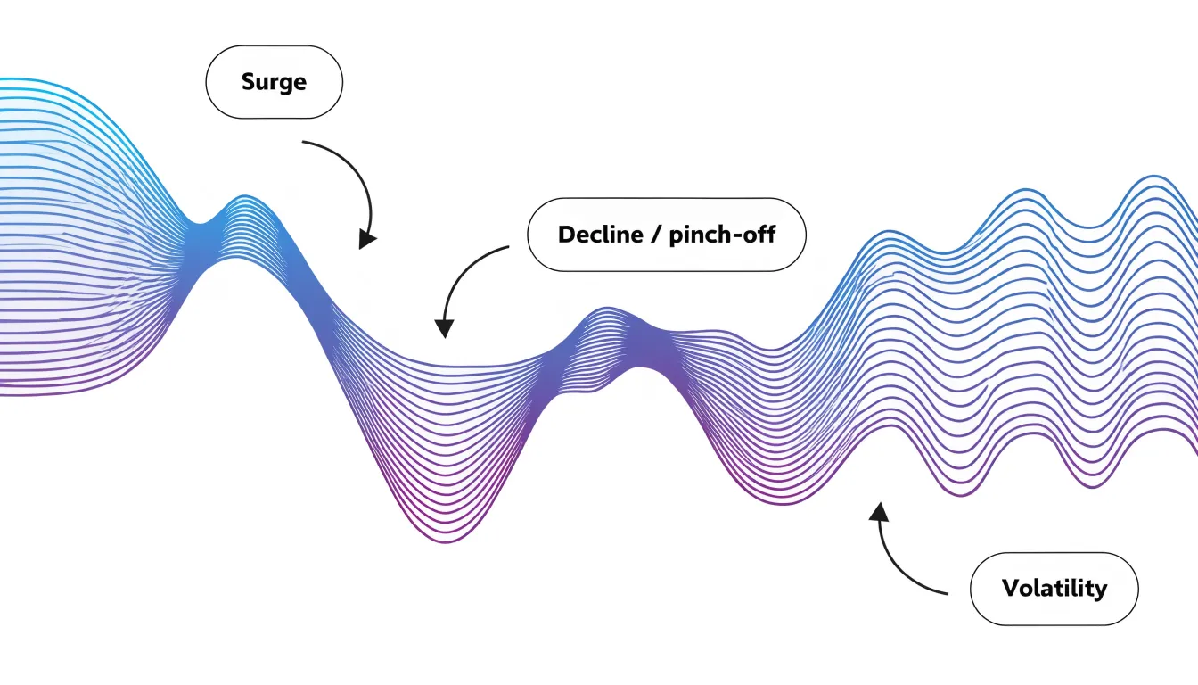
Instead of anchoring every category to a flat axis, the offset baseline keeps the aggregate flow centered, letting each stream expand and contract in both directions. This arrangement emphasizes relative dominance: when one stream grows, surrounding streams are displaced, making the shifting balance of power visible in the overall silhouette.
These shapes highlight transitions across sequential periods:
- Rippling bands indicate a category that rises and falls repeatedly, signaling volatility.
- Steadily widening bands show sustained growth and encroaching dominance.
- Smooth curves between data points soften abrupt changes without hiding them, conveying momentum and direction.
Stream Graph
Stream graphs work well for long-horizon datasets where individual values matter less than the broad movement of the collective:
- Music streaming: A platform tracking genres across a decade can show hip-hop’s band swelling while rock’s narrows, seasonal spikes rippling through holiday music, and new micro-genres emerging from the baseline.
- Website traffic sources: Marketing teams can track organic search, paid campaigns, social referrals, email, and direct visits over months or years to see whether a traffic peak came from a single channel or a broad lift across several.
- Product portfolio sales: Companies can watch how revenue distributes across product lines over multi-year periods, spotting when a flagship line plateaus and a newer offering takes over.
In each scenario, the value comes from pattern recognition at scale: spotting surges, declines, crossovers, and seasonal rhythms across a crowded field of categories.
Stream Graph
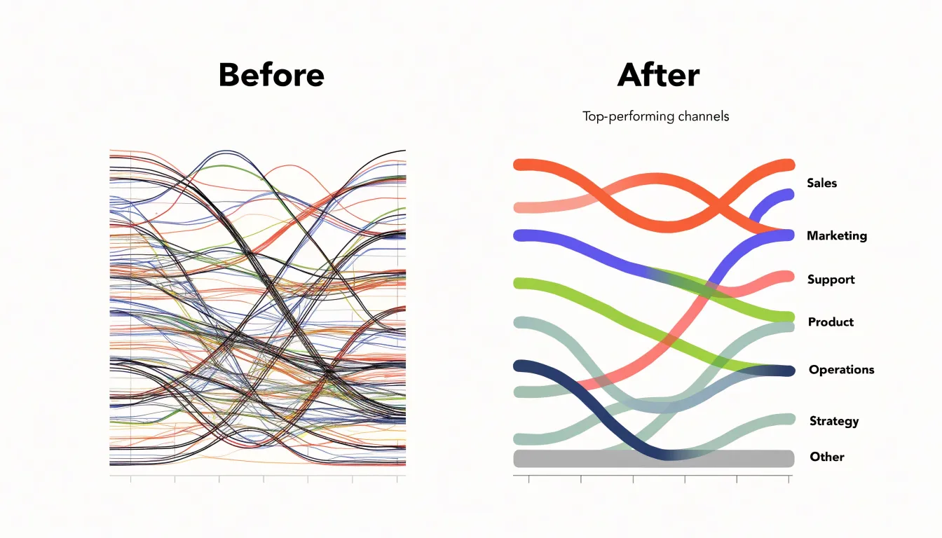
Too many active streams turn the central band into a dense mass where individual shapes are impossible to track and legend matching fails. A workable rule of thumb is to keep roughly five to eight named streams visible at any time. Beyond that count, colors become hard to distinguish and the vertical ordering shifts too frequently to follow.
Two strategies help manage category count:
- Thresholding: A minimum value threshold removes categories whose contribution falls below a chosen level, either across the entire time range (static) or at each individual time step (dynamic). Static thresholds are simple to communicate, while dynamic thresholds adapt to local peaks and valleys but can cause streams to appear and disappear mid-chart. Always state the threshold in the caption so readers know small categories were omitted.
- Grouping into an “Other” layer: Rather than discarding small contributors, sum their values into a single residual stream. This preserves the overall total while reducing the number of shapes. Place the Other layer at one edge of the stack so it does not interrupt the ordering of named streams.
Stream Graph
Shifting the reference line from a flat zero to a curved central path creates a balanced silhouette, but this aesthetic gain comes with a perceptual cost. When the baseline curves, the height of a stream no longer corresponds directly to its absolute value. Viewers must judge a category’s size by its vertical thickness rather than its distance from a fixed axis.
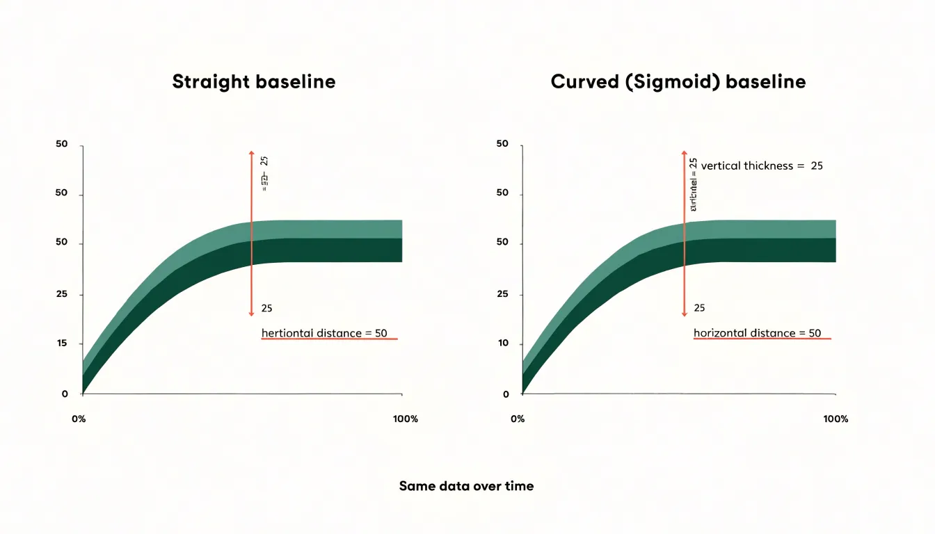
Comparing values across time or between categories becomes difficult because the entire stack flexes with the cumulative total. This distortion is especially pronounced for categories in the middle of the stack, whose positions shift up and down as surrounding layers change. Viewers must mentally reconstruct a local zero to estimate values—a task that grows harder as curvature increases.
Stream Graph
Several additional fields use stream graphs to track competing categories that sum to a meaningful whole:
- Political campaign analysis: Tracking support or fundraising across candidates or issues, revealing surges and collapses that might be missed in a table.
- Finance: Visualizing asset allocation changes to show how capital moves between sectors or asset classes while preserving total portfolio size.
- Digital audience engagement: Charting how users interact with different platform features or content categories over time.
Because the centered baseline emphasizes relative shifts, a category can visibly grow even as the total volume remains flat, highlighting patterns of substitution and dominance.
Stream Graph
Because the curved baseline obscures exact numbers, viewers must rely on relative impressions. Consequently, stream graphs are best used for exploratory overviews and communicating general patterns, not for tasks that require precise data retrieval.
Stream Graph
Because each layer’s vertical position shifts with changes in the layers beneath it, a single turbulent stream can ripple outward and distort the perceived magnitude of its neighbors. Layer ordering is the primary lever for controlling this distortion:
- Centering stable or large streams: Placing low-volatility or high-volume streams near the center of the stack keeps the core silhouette calm. High-volume streams absorb small fluctuations without transmitting them to distant layers, while low-volatility streams create a smooth spine against which erratic outer layers can be read.
- Ordering by magnitude: Sorting layers from largest at the center to smallest at the edges places the biggest contributors along the most stable axis and pushes smaller streams to the peripheral positions.
- Statistical orderings: Sorting by variance, mean value, or correlation between adjacent streams places series that move together beside one another so their shared motion cancels rather than compounds.
- Onset time or thematic grouping: Ordering by when a category emerges or by theme trades modest distortion for narrative coherence and easier tracking of related categories.
In practice, the best orderings often combine these heuristics through iterative visual inspection, keeping the central band steady and pushing volatility toward the margins.
Stream Graph
Because each stream sits directly against its neighbors, colors that are too close in hue or value will blur the boundaries between bands. Varying lightness as well as hue—such as alternating light and dark shades across the stack—keeps adjacent boundaries distinct.
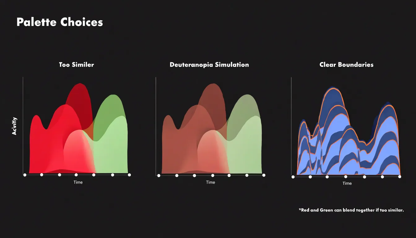
Accessibility requires equal attention:
- Color vision deficiency: Roughly one in twelve men has some form of color blindness, most commonly affecting red and green distinctions. Avoid palettes built on a red-green axis; instead, use combinations that remain distinguishable under deuteranopia and protanopia simulations, such as blue and orange pairings or luminance variations.
- Contrast for low-vision audiences: Pale tints against a white background can fade on low-quality screens or in print. Maintain a clear separation in perceived lightness between adjacent bands and against the background.
- Cognitive load: Limit the palette to a manageable number of distinct colors so viewers do not have to hold too many category mappings in memory. Adding direct labels on or near the streams provides a non-color cue and reduces reliance on a separate legend.
Stream Graph
Interactive tooltips compensate for the lack of precision in a static stream graph. To build an effective interaction layer:
- Add dynamic hover effects: Attach a single
mousemovelistener to the chart container, convert cursor coordinates into the nearest data index using the chart’s scale functions, and highlight the corresponding vertical slice. Slightly dimming unselected bands while raising the active band’s opacity gives immediate feedback without redrawing the entire canvas. Throttle updates withrequestAnimationFrameto keep interactions smooth. - Provide precise data callouts: Name the band under the cursor, report its exact value at that time step, and include the cumulative total for the slice. Format numbers with consistent units and rounding. Anchor the tooltip near the cursor, flipping its placement near chart edges to avoid clipping. Include keyboard focus support so users can step through time intervals using arrow keys.
- Include localized metrics: Add two or three compact contextual figures—such as change from the previous period, percentage share of the total at that moment, or a short trend label—while keeping font size and contrast legible against the underlying colors.
Stream Graph vs Heatmap
Choosing between a stream graph and a heatmap depends on the temporal structure of your data and the patterns you need to reveal. Stream graphs depict continuous temporal flow, showing how parts of a whole shift in volume and proportion over time.
Heatmaps, in contrast, are built for dense, grid-based pattern recognition. They map values to color gradients across a matrix of rows and columns, where each discrete cell represents the intersection of two variables (such as hourly activity across days of the week). This format excels at revealing clusters, outliers, weekly cycles, and hotspots, allowing precise comparisons between individual data points that a continuous stream graph cannot support.
Stream Graph
In newsrooms and media research, stream graphs are used to map how public attention shifts across competing narratives:
- Election coverage: Editors track the relative volume of reporting on healthcare, immigration, the economy, and foreign policy across months of campaigning, revealing how focus drifts from primaries to general elections and how unexpected events swell one topic’s share. This helps newsrooms allocate reporting resources.
- Viral search trends: Analysts studying Google Trends data compare weeks or months of search volume to see the overlapping lifespans of celebrity scandals, natural disasters, or new technologies, identifying which topics cannibalize attention and which sustain interest.
- Archival research: Media researchers map decades of news data on climate change, public health, or economic inequality to expose seasonal patterns, sudden shocks, and slow structural shifts.
Stream Graph
Before committing to a stream graph, run through this checklist:
- Dataset continuity: Ensure your data sits on a continuous axis. If data points are irregular, sparse, or tied to discrete events, smooth interpolation will invent volume that never existed.
- Category count: Keep series to a modest set, typically five to eight, so the silhouette reads clearly and bands remain distinguishable.
- Audience analytical maturity: Because shifting baselines make value estimation harder, confirm your audience is comfortable reading flow and composition rather than looking for standard axes.
- Precision requirements: If readers need to look up exact numbers, trace individual series precisely, or make sharp quantitative comparisons, use a regular stacked area chart or a line chart instead.
Frequently Asked Questions
What is a stream graph used for?
A stream graph is a variation of a stacked area chart that shows changes in category volume over time through an organic, flowing shape. Each category appears as a layer stacked vertically along a continuous time axis, with vertical thickness corresponding to the category’s value at that point in time.
How do you read the horizontal axis and vertical thickness in a stream graph?
The horizontal axis encodes time from left to right, and the spacing between gridlines or tick marks shows the duration each segment represents. Vertical thickness carries each category’s magnitude at a given moment, so compare thicknesses at the same horizontal position to see relative proportions.
How many streams should a stream graph show?
A workable rule of thumb is to keep roughly five to eight named streams visible at any time. Beyond that count, colors become hard to distinguish and the vertical ordering shifts too frequently to follow.
How can I handle too many categories in a stream graph?
Two strategies are thresholding and grouping small contributors into an “Other” layer. If you use thresholding, always state the threshold in the caption so readers know small categories were omitted.
Why can a curved baseline make a stream graph harder to read?
When the baseline curves, the height of a stream no longer corresponds directly to its absolute value, so viewers must judge size by vertical thickness rather than distance from a fixed axis. Comparing values across time or between categories becomes difficult because the entire stack flexes with the cumulative total, especially for categories in the middle of the stack.
When should I use a stream graph instead of a heatmap?
Stream graphs depict continuous temporal flow, showing how parts of a whole shift in volume and proportion over time. Heatmaps are built for dense, grid-based pattern recognition and excel at revealing clusters, outliers, weekly cycles, and hotspots across a matrix of rows and columns.
Tony Astor
Tony writes about data visualization and the tools people use to build charts and dashboards. More about Data Illustrator