Stacked Area Chart vs Stream Graph: Which to Use
 By Tony Astor ·
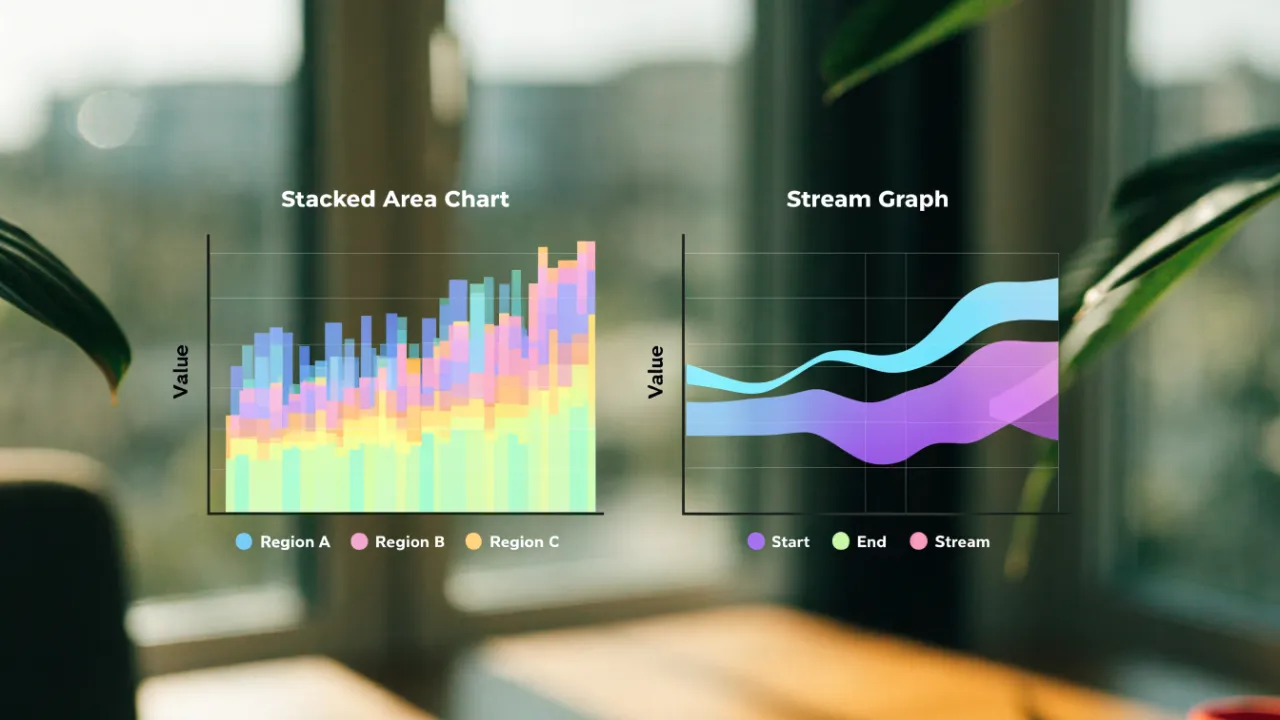
Stacked Area Chart vs Stream Graph
A stacked area chart plots categories on a fixed zero baseline, so band thickness and total height can be read accurately against the y-axis. A stream graph centers layers on a shifting algorithmic axis, emphasizing overall flow and composition rather than precise values. Choose stacked area for exact figures; stream graph for trend and silhouette.
Table of Contents
Stacked Area Chart
A stacked area chart places every category directly on top of the one below it, so the filled bands build upward from a shared starting line. That fixed zero baseline anchors the entire visual structure. Each category’s value is drawn as the vertical distance between its lower and upper edges, and those distances accumulate as the stack rises. The topmost line of the stack therefore traces the grand total across the timeline, giving readers an immediate sense of how the whole evolves from one period to the next.
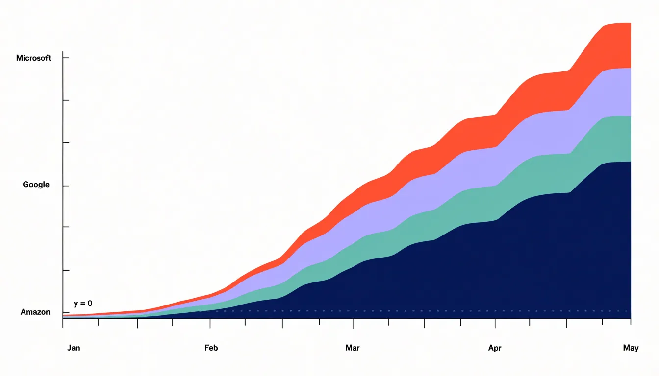
With zero as the common reference, every band’s thickness corresponds directly to its own value, and the overall height corresponds to the combined total. Readers can scan the silhouette of the chart to follow the sum over time, then drop their gaze into the interior to see which band expanded or contracted. A widening band in the middle of the stack shows a category gaining share; a narrowing band shows it receding, even while the total continues to climb.
This arrangement excels when the story involves both aggregate growth and shifting composition. A company tracking revenue by product line, for instance, can show total sales rising across quarters while individual products trade prominence. The continuous horizontal axis reinforces the sense of flow, since adjacent time points connect through unbroken shapes rather than discrete bars.
The trade-off is that only the bottom layer rests on a flat reference. Bands higher in the stack sit atop undulating surfaces, so comparing their absolute heights from period to period requires careful reading. The chart works best when the cumulative total matters as much as the parts, and when the number of categories stays modest enough that each band remains legible.
Stream Graph
Stream graphs arrange data around a central axis that itself shifts and bends, creating a symmetrical, flowing shape that resembles a river or a landscape. This organic aesthetic emerges from allowing the baseline to vary rather than fixing it at zero. Each category’s thickness still represents its value, and the overall form rises and falls as totals change over time, drawing the eye along smooth contours rather than inviting readers to measure against a fixed grid.
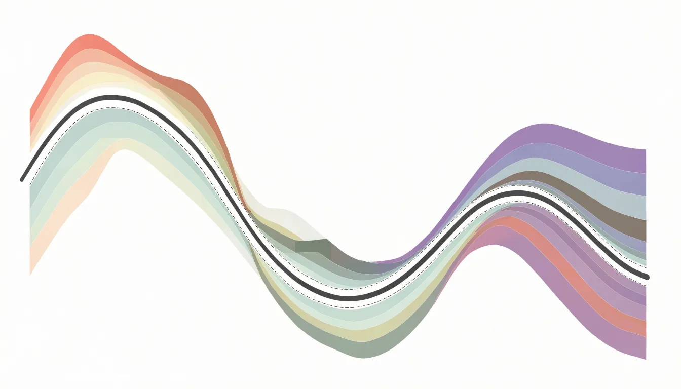
Because the central axis moves, the vertical position of any category at a given moment reflects both its own value and the values of the categories beneath it. This design shifts attention toward macro-level patterns: the swelling and narrowing of the whole stream, the relative dominance of different bands as they widen or thin, and the points where one flow overtakes another. The eye naturally traces the overall rhythm—periods of expansion, contraction, and crossover—without being anchored to exact numerical sums at each time step.
Stream graphs work well for showing how multiple series evolve together in a compact space, especially when the story lies in the changing composition and general trend rather than precise totals. Viewers can quickly grasp which categories grow or shrink and how the balance among them changes, making stream graphs a strong choice for exploratory or narrative visualizations where the big picture matters most.
Baseline Mechanics
The two charts diverge in how their baselines are constructed. In a stacked area chart, every layer rests on a horizontal axis fixed at zero. The bottom edge of the lowest series aligns with the x-axis, enforcing a grounded, hierarchical structure where the first series acts as a foundation and subsequent layers stack sequentially upward. Visual weight is distributed from the bottom up.
In contrast, a stream graph displaces the baseline from the bottom and typically computes it algorithmically to minimize wiggle or center the overall shape around a horizontal midline. Each series is offset from this central axis, and the areas expand both upward and downward. Structurally, the stream graph’s baseline is a derived, dynamic curve that shifts with the data, whereas the stacked area chart’s baseline is a static zero line.
Reading the Charts
These two layouts call on different habits of attention. In a stacked area chart, the viewer traces a band between two boundaries and reads its vertical extent at any horizontal position as a quantity. Because the baseline sits flat along the bottom of the plot, the eye can follow a single category upward through the stack to see how its contribution combines with the layers beneath it, and the top edge of the whole stack gives the accumulated total directly against the y-axis. Readers accustomed to ordinary line charts find the decoding effort modest.
With a stream graph’s stack centered on a moving axis, the viewer can no longer read a band’s thickness against a stationary scale. Reading becomes a matter of gauging relative thickness at a glance and noticing how bands swell, thin, and drift up or down from left to right. Movement itself carries meaning: a band drifting away from center draws the eye and signals emphasis, while a thinning ribbon suggests decline. The stream graph rewards quick perceptual scanning of relative change and directional flow, whereas the stacked area chart rewards careful measurement and accounting of accumulated quantities.
Visual Clarity
Visual clarity hinges on how easily a reader can extract specific values and compare magnitudes across categories. Stacked area charts offer a direct reading experience: a reader can place a finger on a date, trace upward to the top of a given band, and estimate its magnitude or the cumulative total with reasonable confidence. This suits straightforward quantitative retrieval, where someone needs to know how much of something existed at a specific moment.
Stream graphs trade that precision for visual engagement. Their shifting contours emphasize the overall silhouette, making it easy to absorb the gestalt of the chart quickly in exploratory contexts and presentations. Because band thickness varies on both sides of the centerline, estimating a single category’s value requires comparing two moving edges, and a band’s vertical position no longer maps neatly to a number. Readers gain high-level pattern recognition while losing the ability to answer precise quantitative questions with confidence.
Negative Values
Neither design copes well with below-zero data. In a stacked area chart, where each category is drawn on top of the cumulative total beneath it, negative values break the stacking logic: the baseline for subsequent layers shifts downward, and the visual relationship between layers no longer reflects each category’s magnitude. A segment that dips below zero can overlap with the layers above it, creating ambiguous regions where viewers cannot tell which category is responsible for a given area. The apparent thickness of a band may shrink or grow in ways that contradict the underlying numbers. Because the cumulative sum can cross zero, the visual baseline runs through the middle of the plotted regions rather than sitting at the bottom edge.
In a stream graph, the centering algorithm assumes non-negative quantities. A below-zero metric forces the baseline to warp, disrupting the symmetry the design depends on and producing exaggerated bulges and awkward crossings that distort both the negative series and its neighbors. Viewers also lose the intuitive reading of area as magnitude, since the central axis no longer represents zero in a consistent way. Both chart types therefore require values that stay at or above zero; negative metrics call for a different visual approach altogether.
Best Use Cases
Stacked area charts fit settings where an audit trail, budget review, or capacity plan depends on the numbers themselves:
- Financial reporting: A viewer can trace the height of a single band against the y-axis to recover a specific revenue figure for a product line, region, or quarter.
- Inventory tracking: A warehouse manager can see the absolute stock level of each category on a given date alongside total holdings, comparing component sizes across time periods without recalculation.
Stream graphs suit large, energetic datasets where viewers want to sense where activity is concentrated and how it moves:
- Music listening trends: The ebb and flow of genres across months produces a silhouette that reveals surges in popularity, seasonal shifts, and emerging styles.
- Social sentiment data: Conversation volume around topics or hashtags rises and falls in waves that are easier to perceive as a continuous band than as separate lines.
- High-volume event logs, web traffic by channel, and streaming engagement metrics: Smoothed, centered bands emphasize momentum and relative proportion over exact figures.
The Perception Problem
Human vision is good at comparing straight, aligned edges, and poor at comparing curved, undulating boundaries. In a stream graph, judging the vertical distance between two moving curves at an arbitrary horizontal position is harder than it appears. Without a reliable internal ruler for curved extent, the eye estimates distance by comparing shapes, and shifting reference points lead viewers to consistently under- or overestimate band thickness—with errors growing as curvature increases.
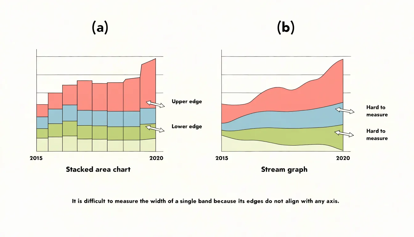
Stream graphs also introduce optical illusions familiar from the study of filled shapes:
- Size assimilation: Slender bands that bulge outward can appear thinner than they are, especially next to a thick neighboring band.
- Midpoint drift: Bands whose upper and lower edges curve in opposite directions create a lens-like shape whose apparent midpoint drifts away from the true midpoint.
- Figure-ground ambiguity: Rounded corners and a symmetric, flowing silhouette can lead viewers to read the outline of the whole shape rather than individual bands, losing track of where one series ends and another begins.
As a consequence, fine distinctions disappear. Two bands differing by a few percentage points may look identical, while a band that changes only slightly can appear to swell or shrink dramatically depending on its neighbors’ slope. Viewers who need exact values must rely on tooltips or labels rather than their eyes.
Sorting Categories
The order in which categories are stacked shapes how a chart reads, because every series inherits the vertical motion of everything beneath it. When lower layers fluctuate, that inheritance turns small variations into visible wobble, and the topmost series can appear to swing dramatically even when its own values barely change. Choosing a deliberate order rather than accepting the source data’s sequence gives the chart a calmer, more faithful shape:
- Low-variance series near the baseline: Stable bands form a quiet foundation, so the top silhouette is driven mainly by series that genuinely vary, reducing visual noise.
- Grouping related categories: When neighboring series rise and fall together, their shared boundaries stay comparatively smooth and the overall contour is easier to follow.
- Ordering by average magnitude (largest at the bottom): Substantial, steadier bands anchor the chart and keep smaller categories legible.
Whatever rule is adopted should be applied consistently and stated in the legend or caption so readers understand the arrangement.
Color Choices
Because adjacent bands sit directly against one another, their boundaries must remain legible at every point along the horizontal axis. Colors should differ enough in hue or lightness for neighboring layers to separate cleanly, including for viewers with color vision deficiencies. Colorblind-safe palettes and contrast checkers help confirm that layers remain distinguishable at small sizes or on different screens.
Assigning colors so that adjacent bands contrast strongly in lightness makes the boundary between them read almost as a line, helping viewers follow a single layer from left to right. Muted, closely related shades can blur boundaries and invite misreading. At the same time, a dozen highly saturated colors will compete for attention; limiting saturation and reserving the strongest colors for the most important layers keeps focus on the data while letting the overall flow remain clear.
Interactive Features
Interactive features overcome the precision limits of area-based charts, turning a qualitative overview into a quantitative tool:
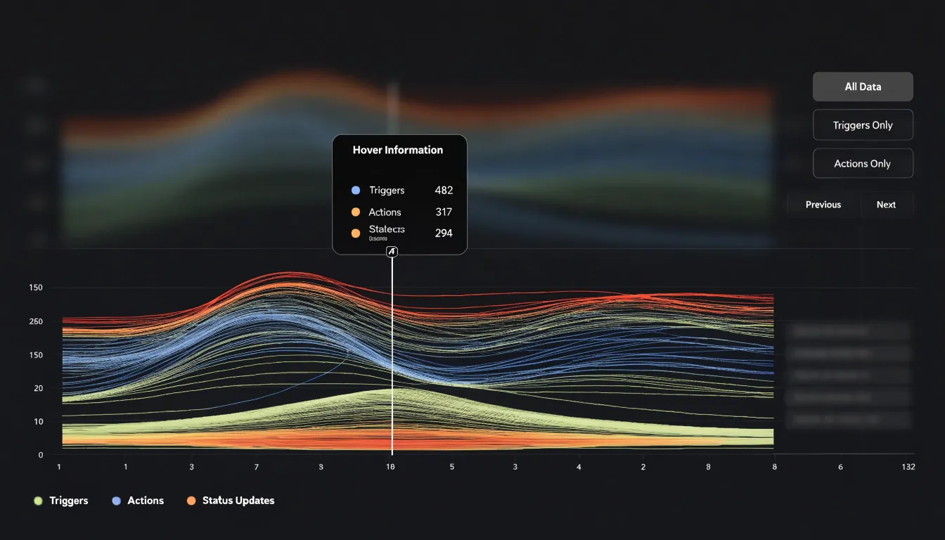
- Tooltips and hover states: Moving the cursor over a specific x-axis position—such as a single month in a revenue chart—reveals the exact numerical values or band thickness for each category, along with added context like percentage changes or comparisons to previous periods.
- Click-to-filter legends: Clicking a legend item isolates selected series and dynamically updates the chart, reducing visual clutter so tooltips and visual comparisons focus on that series alone.
Hover interactions are especially critical in stream graphs, where the moving baseline prevents users from estimating values against an axis.
Common Design Pitfalls
- Overcrowding with too many categories: Including a dozen or more series makes each layer thin and indistinguishable, especially when colors are similar or hierarchy is unclear. Focus on the most relevant categories rather than plotting every available series.
- Poorly placed inline labels: Labels inserted directly into bands often overlap with adjacent layers when values fluctuate, become unreadable where a band narrows or disappears, or collide at the ends of converging bands.
- Unsmoothed data spikes: Sudden, sharp spikes from anomalies or natural volatility create jagged edges that disrupt continuous flow and make the chart look erratic. Where exact raw values are not required, smoothing techniques such as moving averages or spline interpolation can preserve readability.
Performance and Scalability
When a chart carries into the twenties or thirties of series, each additional stream adds polygons to render, legend entries to manage, and hover targets to track. The first defense is reducing cardinality at the data level by grouping the long tail of minor categories into a single “Other” bucket, which keeps the chart legible while preserving total magnitude. Common thresholds include ranking series by maximum or average value and keeping a fixed count, a percentage of the total, or the categories that account for 90% of the volume.
On the rendering side, several optimizations keep interactions fluid:
- Flatten expensive effects—smoothing curves, drop shadows, and individual gradients—during interactions to reduce frame-by-frame work.
- Avoid redrawing the entire chart on pointer movement; update only the affected layer or render highlights on a separate overlay.
- In SVG, consolidate series into fewer path elements, or switch to canvas when stream counts are high.
- Virtualize or debounce expensive recomputations such as re-sorting series or recalculating stacking order, and test early with realistic data volumes.
Quick Decision Matrix
Use four parameters to choose between the two formats:
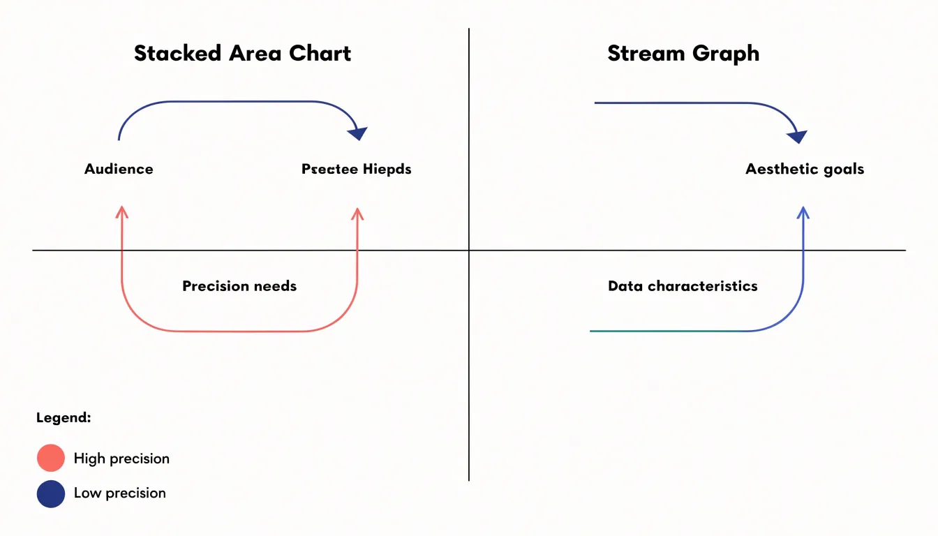
- Audience: Analysts and stakeholders who need to trace individual categories and read exact figures are best served by a stacked area chart. General audiences or presentation settings where overall flow matters more than exact numbers suit a stream graph.
- Precision needs: Budget allocations, cumulative totals, and accurate comparisons require the stacked area chart’s consistent baseline. Trend exploration tolerates the vertical shifts of a stream graph.
- Aesthetic goals: Stacked area charts provide a clean, conventional look for standard business reporting. Stream graphs offer a striking, modern graphic that emphasizes the ebb and flow of multiple series.
- Data characteristics: Fewer categories with a clear hierarchical structure fit a stacked area chart; many categories with subtle variations often benefit from a stream graph’s centered layout.
Final Selection Guide
To integrate these charts into a visualization workflow:
- Define the question: Decide whether you are comparing parts to a measurable whole (stacked area) or highlighting the evolution of a shifting mix (stream graph).
- Prepare the data: Ensure consistent categories and clear labeling for stacked area charts; apply smoothing and cap the category count for stream graphs.
- Account for audience familiarity: Provide extra explanation when using stream graphs, along with clear titles, annotations, and accessible colors.
- Test and document: Review the draft with a small group to confirm it reads without confusion, and record your selection rationale to maintain consistency across projects.
Frequently Asked Questions
What is the difference between a stacked area chart and a stream graph?
A stacked area chart uses a fixed zero baseline and stacks every category upward from it, while a stream graph uses a shifting central axis and typically computes its baseline algorithmically to center the overall shape. In a stream graph, areas expand both upward and downward from that derived baseline.
When should I use a stacked area chart instead of a stream graph?
Use a stacked area chart when viewers need to trace individual categories and read exact figures, such as budget allocations, cumulative totals, or financial reporting. Stream graphs suit general audiences or presentation settings where overall flow matters more than exact numbers.
Can stacked area charts or stream graphs show negative values?
Neither design copes well with below-zero data. Stacked area charts and stream graphs both require values that stay at or above zero, and negative metrics call for a different visual approach altogether.
Why are stream graphs harder to read precisely?
Stream graphs use a moving central axis, so estimating a single category’s value requires comparing two moving edges, and a band’s vertical position no longer maps neatly to a number. Viewers may also under- or overestimate band thickness as curvature increases.
How should I sort categories in a stacked area chart?
Use a deliberate order rather than the source data’s sequence: place low-variance series near the baseline, group related categories, and order by average magnitude with the largest at the bottom. Apply the rule consistently and state it in the legend or caption.
How can I read exact values in a stream graph?
Hover interactions are especially critical in stream graphs because the moving baseline prevents users from estimating values against an axis. Tooltips and hover states can reveal exact numerical values or band thickness for each category at a specific x-axis position.
Tony Astor
Tony writes about data visualization and the tools people use to build charts and dashboards. More about Data Illustrator