Spiral Plot: Showing Cyclical Patterns Over Time
 By Tony Astor ·

Spiral Plot
A spiral plot is a data visualization that wraps a repeating time series around a central point, with angular position representing phase within a cycle (such as hour, week, or month) and radial distance representing time progression across cycles. Aligning equivalent phases on the same radial line lets viewers compare cycles and spot patterns, anomalies, and trends at a glance.
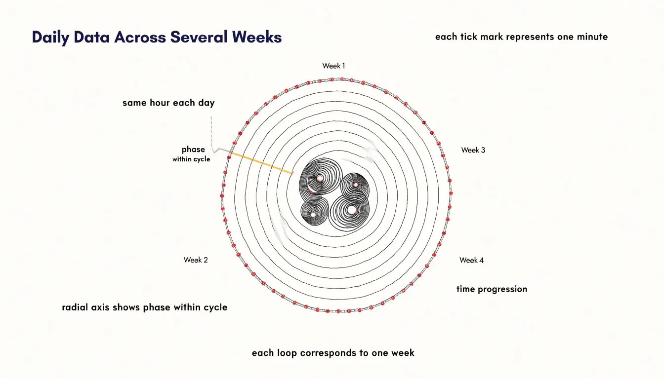
Table of Contents
Spiral Plot
Fixed-length time segments arranged along a shared radial axis transform repetition into something the eye can grasp immediately. Each day, week, or year becomes an arc of the same angular width, and every cycle is drawn on a common radius that starts at the same angular position. This shared starting line works like the zero mark on a clock: sunrise, Monday morning, or January first always lands at the same angle, so the viewer’s gaze moves outward through consecutive cycles along a predictable path. Because each segment occupies an identical angular span, a point at three in the afternoon on one turn sits directly beyond three in the afternoon on the previous turn. Reading outward along any radial line compares the same moment across many cycles, and the recurrent shape of the data becomes visible without any mental arithmetic.
Regular rhythms announce themselves as continuous streaks running outward from the center, while departures from routine appear as breaks, spikes, or drifts in the band. Commuters see weekday peaks settle into two steady ridges along one half of the circle and quieter weekend arcs along the other. Annual data arranged this way shows winter heating demand or summer cooling load forming repeated seasonal bulges at fixed angles.
The radial layout also compresses a long record into a compact figure, letting hundreds of cycles occupy a single page while preserving the identity of each individual turn. Patterns that would be buried in a linear time series, such as a gradually shifting peak across successive weeks, show up as a spiral drift that the eye follows around successive rings. This combination of constant angular spacing and a shared radial reference turns cyclical data into a visual rhythm where daily, weekly, and annual behavior stand out through the geometry alone.
Spiral Plot
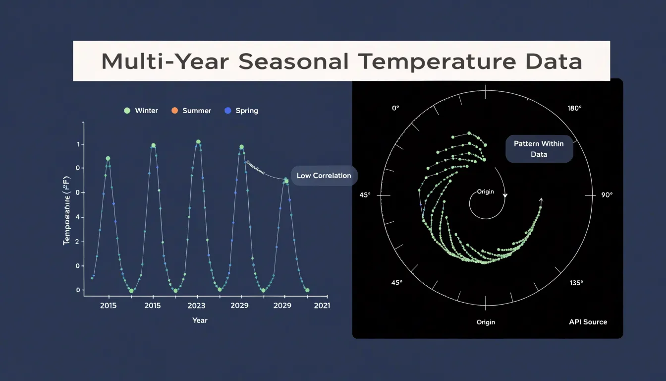
Traditional horizontal timelines arrange time along a single axis, stretching events from left to right in an unbroken line. This works well for one-off sequences, yet it struggles when the data contains repeating cycles. When a horizontal graph displays a periodic process such as a seasonal pattern, a biological rhythm, or a recurring economic indicator, the same phase of the cycle appears at scattered positions across the chart. The spring peak in one year sits far from the spring peak of the next, separated by the accumulated width of all intervening months. To compare them, a reader must trace across the page, remember the position of the earlier point, and mentally overlay the two. Each additional cycle adds more distance, and the correspondence between equivalent moments grows harder to perceive.
Wrapping the timeline around a central axis resolves this distance problem. Because points that occupy the same phase of successive cycles stack into a radial column, the spring peak of every year lines up directly above or below its counterparts, forming a visible spoke. This alignment turns comparison into a matter of reading along a spoke rather than scanning across a wide horizontal span. Consistent rises at a particular week or repeated dips at a fixed interval emerge as clear visual ridges or troughs along the spiral’s coils.
The circular arrangement also preserves a sense of continuity. A horizontal timeline implies a beginning and an end, while a spiral suggests ongoing repetition that nonetheless advances over time. The outward drift of the coils encodes progress, and the angular position encodes phase within the cycle, allowing both dimensions to be read at once. Readers can follow a single loop to understand one period, then compare loops to spot long-term shifts.
Spiral Plot
Reading a spiral plot begins with identifying which visual channel carries each variable. Radial distance from the center typically encodes time progression, so a point near the center represents an early observation and a point farther out represents a later one. Tracing a line outward moves forward chronologically, and the spacing between successive turns shows how densely observations are packed. Angular position encodes the position within a repeating cycle, such as the hour of a day, the month of a year, or the phase of a periodic process. A full rotation through 360 degrees corresponds to one complete cycle, and the starting angle marks the boundary between one cycle and the next.
Data magnitude appears through line width or color intensity rather than through position. A thicker stroke or a more saturated shade signals a larger value, while a thinner or paler line signals a smaller one. These channels work in parallel with the radial and angular axes, so a single segment of the spiral can convey all three dimensions at once: where the observation sits in time, where it falls inside its cycle, and how large it is.
Reading the plot accurately means separating these roles. Follow the radius to locate the moment in the overall sequence, follow the angle to place it within a repeating period, and read the stroke’s width or color to judge its magnitude. Comparing rings across turns reveals how the same phase of a cycle changes from period to period, and comparing widths along a single ring reveals variation within a cycle. Checking where a line grows thicker or shifts color as it moves outward gives a quick sense of when a quantity rises or falls over time.
Spiral Plot
Multi-year environmental and operational datasets often span stretches of time that obscure recurring patterns on a conventional linear axis. Mapping each year to one full revolution turns the calendar into a spatial scaffold, letting the eye follow the cyclic rhythm of the year while reading the progression of years outward from the center.
Weather data illustrate the value of this layout. Daily temperature, rainfall, or wind measurements collected across a decade can be mapped so that each January sits at the same angle on every loop, causing the cold season to form a vertical ridge running outward through the spiral. Seasonal activity peaks, such as monsoon onset, spring bloom, or the timing of peak energy demand, become immediately legible as denser coloration or sharper transitions at consistent angular positions. Anomalies stand out too: a year in which a heatwave arrives weeks early produces a band that bends away from the established radial line, drawing attention to the deviation without obscuring the underlying norm.
Operational datasets benefit from the same treatment. Shipping volumes, visitor counts, maintenance tickets, or sensor readings accumulate over years and typically carry strong seasonal components. Wrapping these records annually reveals recurring surges and lulls as stable features of the spiral, while multi-year trends appear as gradual changes in band width or color intensity from inner loops to outer ones. Analysts can thus distinguish a one-off disruption from a genuine shift in seasonal behavior.
Spiral Plot
When a spiral plot arranges 24-hour daily cycles along a continuous monthly spiral, each loop represents one day and successive loops step outward or inward as the month advances. Midnight, dawn, midday, and dusk always occupy the same orientation on the page, so patterns that unfold across weeks appear as coherent shapes instead of isolated data points on separate daily charts.
Plotted this way, recurring personal behaviors emerge clearly. A block of activity at the same hour each day draws a radial band running outward through successive loops, while irregular events scatter across the spiral. Long-term habits show up as thick, continuous ribbons that persist through the month, revealing how firmly a routine is anchored. Shifting sleep patterns appear as bands that drift gradually in angle from one loop to the next, making it easy to see bedtime or wake time sliding later across weeks, and to connect that drift to weekends, deadlines, or seasonal changes in daylight.
Lifestyle consistency is visible in the overall regularity of the spiral. A month with stable routines produces clean, evenly spaced bands and predictable transitions, whereas a disrupted month shows broken bands, gaps, and erratic placement of activities. Because the spiral preserves adjacency between one day and the next, transitions at the boundary between days remain visible, so late-night activity flows naturally into the following morning. This makes the spiral plot a compact instrument for auditing personal rhythms, comparing months against each other, and identifying the moments when daily structure begins to erode or stabilize.
Spiral Plot
Botanical researchers and farmers rely on spiral plots to trace the full arc of a crop’s development across a growing season and beyond. The spiral format allows a continuous visual thread to connect germination phases, vegetative growth, flowering, and harvest into a single readable timeline. Yield volumes can be plotted as the radial width of the band at each point, letting growers see at a glance how harvest output swells and contracts across successive weekly or monthly cycles.
For essential oil crops, the spiral becomes especially useful because harvest timing is tightly linked to oil concentration and plant maturity. A researcher can mark the precise window when lavender or peppermint reaches peak oil content, then compare that window against earlier and later cycles to refine future planting schedules. Germination phases appear as the innermost segments of the spiral, where early sprouting rates and emergence percentages can be logged and compared across seed batches.
Rotating agricultural cycles fit naturally into this geometry, since each full revolution can represent a complete crop rotation, with successive revolutions showing how soil conditions, input costs, and yields shift over seasons. Farmers using the spiral plot can overlay weather data, irrigation logs, or pest observations onto the same curve, revealing correlations that linear charts tend to obscure. The circular form also highlights seasonal overlap, showing where one crop’s harvest coincides with another’s planting, giving agricultural teams a practical tool for planning, benchmarking, and communicating the rhythm of their fields to stakeholders.
Spiral Plot
When values are plotted as marks along the spiral curve, the recurring patterns of a dataset settle into a familiar background rhythm. Against this steady background, unusual events become immediately visible.
An unexpected anomaly appears as a mark that deviates from the position its neighbors occupy on adjacent turns of the curve. Because comparable periods sit side by side, a sudden spike rises visibly above the band of ordinary values, while a sharp drop sinks below it, and both stand out precisely because the surrounding marks follow the established pattern. The continuous curve also makes it easier to trace how an anomaly develops. A gradual rise that accelerates into a spike shows its trajectory along the arc, and a rapid fall that recovers within a single turn remains legible as a distinct dip.
This makes the spiral plot useful for monitoring long-running series, where the volume of data would overwhelm a conventional line chart or make month-by-month comparison tedious. Reviewers can scan the spiral and let the regularity of the background rhythm guide their attention toward the places where it breaks, while the position of each departure along the curve shows exactly when it occurred.
Spiral Plot
Drawing consecutive years as adjacent loops rather than separate panels makes year-over-year comparison a natural reading of the chart. When activity is stable, the loops stack almost on top of each other, and the eye registers the repetition as a calm, regular band. When something changes, the drift shows up as a widening or narrowing gap between successive turns. A slow increase in baseline activity appears as each loop sitting slightly farther out than the last, a gentle outward creep that would be tedious to confirm month by month in a table but is immediately visible as a spiraling expansion. A gradual decline reads the same way in reverse, with each revolution drawing in toward the center.
Subtle structural shifts are also easier to catch. A seasonal peak that once occurred in one month and has begun arriving earlier will visibly rotate around the spiral, its position shifting relative to the loop above it. A change in the shape of the seasonal curve, such as a flattening of the summer trough or a sharper winter spike, becomes apparent when the profile of one revolution is held against the profile of the one just inside it. Because the viewer compares nearby loops rather than distant points, these changes stand out against ordinary seasonal variation, letting analysts distinguish genuine movement in the underlying process from routine annual fluctuation.
Spiral Plot
Color is the primary channel through which a spiral plot communicates intensity, turning an abstract sequence of values into a readable visual gradient along the winding path. A continuous color ramp assigns each data point a position on a scale, so that temperature readings climbing from cool blues through neutral midtones to warm reds reveal their progression at a glance, even as the spiral carries the eye through many rotations. Designers typically choose a perceptually uniform palette so that equal steps in the underlying metric produce roughly equal steps in perceived color, preventing the chart from exaggerating changes in one part of the range while flattening them in another.
Heatmap-style encoding extends this logic across the full band of the spiral: each segment of the path is filled according to its value, producing a ribbon of shifting hue that lets readers scan for hot spots, cold stretches, or abrupt transitions without consulting a legend for every point. Contrasting hues serve a complementary role when the data contains meaningful thresholds or categories. A sharp break from green to amber at a stress score of seventy, for instance, marks the boundary between acceptable and concerning conditions and draws attention to where along the spiral that boundary is crossed.
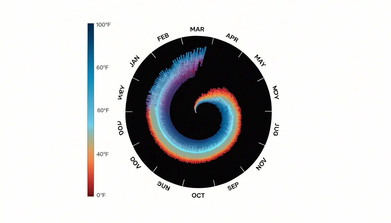
Sequential gradients, diverging schemes centered on a neutral midpoint, and qualitative palettes for discrete states each suit different kinds of quantitative metrics. Because the spiral compresses a long series into a compact area, color also compensates for the reduced space available to individual marks, carrying information that position and height alone might crowd out. Careful calibration of the palette, including checks for color vision deficiency and sufficient lightness variation, ensures the intensity encoding remains legible across the entire sweep of the spiral path.
Spiral Plot
Selecting the correct lap duration is the foundational decision when constructing a spiral plot. The lap represents one full revolution of the spiral, and its length in time determines how data points map onto the radial axis. When the lap duration matches the natural periodicity of the underlying data—such as placing daily cycles on a 24-hour lap or weekly data on a 7-day lap—recurring patterns line up along the same radial vectors across successive turns.
When the lap duration is mismatched, the consequences spread through the entire visualization. A weekly pattern plotted on a monthly lap drifts by a few days with each revolution, so that the same weekday lands on a slightly different angle every turn. The result is a smeared, braided appearance in which genuine structure becomes difficult to separate from the artifact of misalignment. Readers may interpret this drift as a real trend, which undermines the credibility of the chart. Even small errors accumulate quickly, since a half-day offset compounds over dozens of laps.
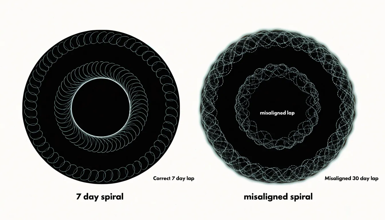
Choosing the scale also involves practical tradeoffs. Short laps such as daily produce many turns and a dense, tightly wound spiral that suits high-frequency data but can crowd the center. Longer laps such as monthly or yearly reduce the number of turns and give each data point more angular room, which helps when the dataset spans several years. The guiding principle is to match the lap to the dominant cycle in the data, then check whether the resulting number of turns keeps the plot legible. A quick visual check for clean radial alignment across turns confirms that the chosen duration is appropriate before the final chart is produced.
Spiral Plot
As the radius of a spiral plot grows, the circumference of each lap increases proportionally. This means that a constant angular span covers a longer arc length on outer laps than on inner ones. If data values are encoded by arc length or if marks are placed at equal angular intervals, the outer laps will appear to carry more visual weight per data point, creating a misleading impression of density and importance.
To avoid this distortion, the mapping from data to angle must be adjusted for the expanding circumference. One approach is to normalize the angular position by the radius, so that equal data intervals correspond to equal arc lengths regardless of lap. Another is to vary the number of data points per lap in proportion to the circumference, keeping the linear density of marks constant. When using area or length to encode values, the scaling must account for the local circumference; otherwise, a value that appears twice as large on an outer lap may actually represent the same quantity as a smaller mark on an inner lap.
Visual weight is also affected by the fact that outer laps have more space, so marks can appear more prominent even when they represent identical values. To maintain accuracy, the designer should consider using constant arc length per data unit, adjusting mark sizes inversely with radius, or explicitly labeling the radial scale and providing reference lines. Additionally, the choice of spiral type—Archimedean versus logarithmic—affects how quickly circumference grows, and thus how severe the distortion becomes. By carefully calibrating the angular and radial mappings, the spiral plot can preserve data density and visual weight across all laps, ensuring that the viewer’s perception aligns with the underlying values.
Spiral Plot
Preparing spreadsheet data for a spiral plot begins with consistent timestamp handling. Store each timestamp in a single column using an ISO-style format such as YYYY-MM-DD HH:MM:SS, and keep time zone information uniform across every row. Spreadsheet software often converts vague date strings into inconsistent serial values, so set the column type explicitly to date-time before exporting. Sorting rows chronologically at this stage prevents gaps and overlaps once the spiral is drawn.
With timestamps clean, calculate the radial angle for each record. A common approach maps the position within a repeating cycle to a full turn: for daily data, take the hour and minute, convert to a fraction of the day, and multiply by 360 degrees. Add a column that stores this angle in radians as well, since many plotting libraries expect radians while spreadsheets default to degrees. Keep one angle column per cycle length you intend to visualise so the same sheet can render hourly, weekly, or monthly spirals without recalculation.
Next, assign a continuous distance variable that controls how far each point sits from the centre. This variable can be a running count of periods elapsed since the first record, scaled by a chosen spacing factor. Use a formula that increments evenly, for example dividing the row index by the number of records per turn, and store the result in its own column labelled radius. Avoid rounding this column too early; retain several decimal places so the curve stays smooth.
Finally, structure the raw CSV so each row carries one observation with columns for timestamp, angle, radius, and value. Keep headers short and free of spaces, remove merged cells and decorative rows, and export as UTF-8. A tidy flat table with one record per line gives plotting tools a predictable input for smooth spiral rendering.
Spiral Plot
Biometric wearables generate a continuous stream of data about the body: heart rate variability, skin temperature, movement, and sleep stages. When that data is plotted on a spiral where each day is a point along the curve and successive rotations represent weeks or months, an individual can spot the weeks when resting heart rate climbed steadily, or the nights when deep sleep collapsed into short, fragmented intervals.
The spiral format becomes especially useful when it is paired with the scheduling of aromatherapy. Someone diffusing lavender oil before bed can mark those sessions directly on the spiral, then observe whether the following nights show longer stretches of restorative sleep. Over several rotations, patterns emerge: perhaps the scent sessions coincide with calmer heart rate variability during the first hours of sleep, or perhaps their effect fades after a few consecutive nights. Because earlier cycles remain visible alongside later ones, this comparison happens without laborious spreadsheet review.
Stress spikes also find a natural home on the spiral. A demanding workweek shows up as a tight cluster of elevated readings, making it easy to trace what preceded and followed that cluster. Individuals can see whether a stressful period was followed by compensatory deep sleep, or whether stress bled into the weekend and disrupted recovery. By connecting aromatherapy schedules, stress markers, and sleep quality on one continuous timeline, the spiral supports informed adjustments to daily routines and relaxation practices.
Spiral Plot
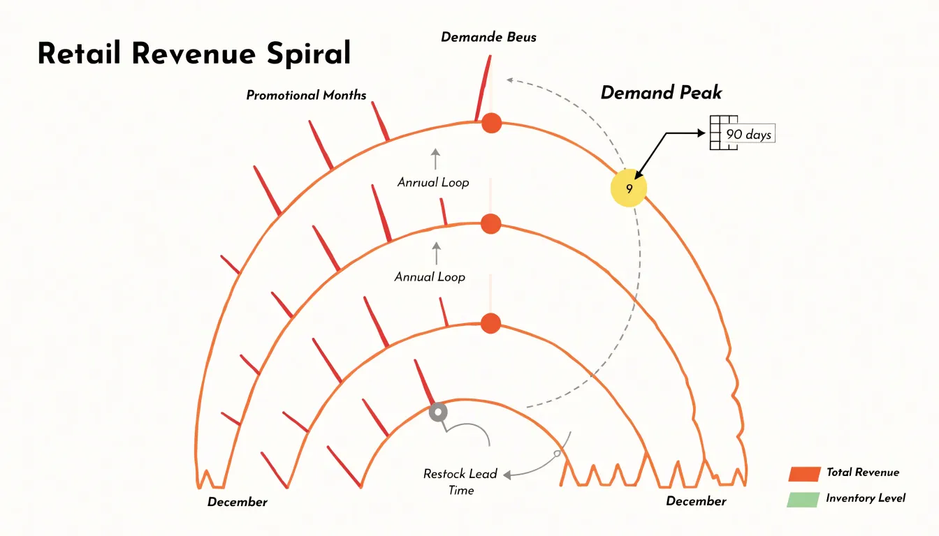
E-commerce and retail brands operate on rhythms that repeat and evolve at the same time. Revenue rises and falls with quarterly reporting periods, promotional events such as holiday sales or flash discounts, and seasonal shifts in customer demand. Wrapping a retail time series into quarterly or annual loops produces a continuous ribbon of data in which comparable months or weeks line up radially.
For inventory planning, this alignment is especially useful. When quarterly revenue is charted along the spiral, planners can compare the current quarter against the same quarter in prior loops and see whether the business is growing, flattening, or contracting. Promotional bursts appear as sharp outward spikes along the ribbon, and their position relative to earlier spikes shows how campaign timing has shifted year over year. Seasonal demand, such as the surge in outdoor goods each spring or the rise in gift purchases each December, forms a repeating ridge that traces a clean arc through the spiral. Deviations from that arc signal anomalies worth investigating, whether a supply delay, a competitor’s price move, or an unexpected change in consumer behavior.
The spiral format also supports inventory optimization directly. By reading the radial distance between demand peaks and the lead times required to restock, teams can calibrate order quantities and safety stock against the cadence the chart reveals. Holding several cycles in view simultaneously lets decision-makers plan promotions, markdowns, and replenishment with a clearer sense of precedent and trajectory.
Spiral Plot
Interactive spiral visualizations gain substantial value when embedded within broader analytical dashboards, where they function alongside other charts, filters, and summary metrics to support exploratory data analysis and executive reporting. Placing a spiral plot within a dashboard context allows analysts to cross-reference cyclical patterns with complementary views such as trend lines, heatmaps, or categorical breakdowns. Analysts can apply dashboard-level filters to focus the spiral on specific regions, products, or time windows, then observe how the cyclic structure shifts in response. This interactivity turns the spiral from a static illustration into a working investigative tool, letting users drill into dense segments, hover for exact values, and compare multiple spiral series side by side.
For executive reporting, the dashboard setting provides necessary context. Executives viewing a spiral plot alongside key performance indicators, summary tiles, and annotated highlights can interpret cyclical movements in relation to targets and strategic priorities. Surrounding dashboard elements supply the quantitative grounding that decision-makers require, while linked interactions strengthen the view: selecting a period on a companion line chart can highlight the corresponding arc on the spiral, and selecting an arc can update other panels to show the underlying detail.
Integrating spiral plots into dashboards also supports collaborative analysis, since shared views and consistent filter states let teams discuss the same visual evidence. Responsive design considerations ensure the spiral remains legible across screen sizes, and clear labeling of cycle boundaries keeps interpretation reliable. When designed with these practices, spiral plots become a natural component of a layered analytical environment, serving both open-ended exploration and structured executive briefings.
Frequently Asked Questions
What is a spiral plot used for?
A spiral plot is used to arrange fixed-length time segments along a shared radial axis so repeating cycles can be compared visually. It can compress a long record into a compact figure while preserving each individual turn.
How do you read a spiral plot?
Radial distance usually encodes time progression, while angular position encodes where an observation falls within a repeating cycle. Data magnitude is shown by line width or color intensity, so you follow the radius for overall sequence, the angle for cycle phase, and width or color for magnitude.
Why use a spiral plot instead of a traditional timeline?
A horizontal timeline struggles when data contain repeating cycles, because the same phase appears at scattered positions across the chart. Wrapping the timeline around a central axis stacks the same phase into a radial column, making comparison easier. It also preserves continuity while showing ongoing repetition and progress over time.
How do you choose lap duration for a spiral plot?
Match the lap duration to the dominant cycle in the data, such as a 24-hour lap for daily cycles or a 7-day lap for weekly data. A mismatched lap can smear or braid the pattern and make real structure hard to separate from misalignment, so check for clean radial alignment across turns.
How do you prepare spreadsheet data for a spiral plot?
Store each timestamp in one column using an ISO-style format and keep time zone information uniform, then sort rows chronologically. Calculate an angle for each record for each cycle length you plan to visualize, and assign a continuous radius variable based on periods elapsed. Export a tidy flat CSV with one observation per row and columns for timestamp, angle, radius, and value.
How are spiral plots used for weather or operational data?
Mapping each year to one revolution turns the calendar into a scaffold, so seasonal patterns such as cold seasons, monsoon onset, or peak energy demand line up at consistent angles. Operational records like shipping volumes, visitor counts, maintenance tickets, or sensor readings can reveal recurring surges and lulls, while multi-year trends appear as gradual changes in band width or color intensity from inner loops to outer ones.
Tony Astor
Tony writes about data visualization and the tools people use to build charts and dashboards. More about Data Illustrator