Small Multiples vs Overlay Chart: Which Compares Better?
 By Tony Astor ·

Small Multiples vs Overlay Chart
Small multiples show each data series in its own small panel sharing identical chart type and axis scales, while overlay charts plot multiple series on one shared axis. Use small multiples for many series or trend comparison across categories; use overlays for two to five series where direct intersections and exact relative positions matter most.
Table of Contents
Small Multiples
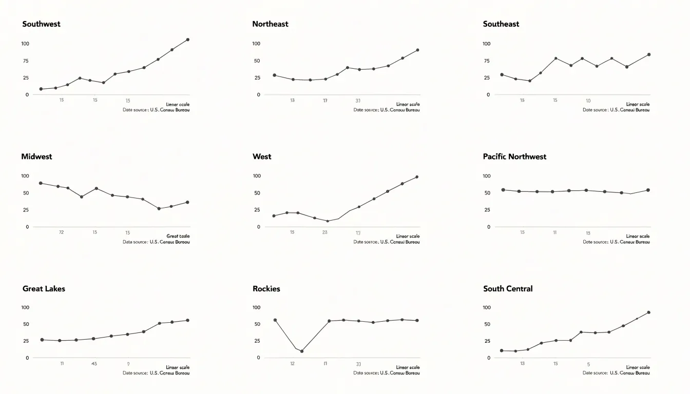
Small multiples present a series of miniature charts arranged in a uniform grid, each panel displaying the same chart type, the same axis scales, and the same visual encoding for a different slice of the data. Because every panel shares identical structure, viewers can scan the grid as a whole while also dropping into any single panel to study one metric in isolation. The grid acts as a comparison engine: the eye moves from panel to panel, picking up differences in slope, level, and volatility without the confusion that arises when many lines are stacked inside one frame. Each metric occupies its own dedicated space, so a spike in one series never hides a dip in another. Axis clutter disappears as well, since each panel carries a clean, shared scale rather than a tangle of competing labels and legends layered over a single plot area. The repeated axes and consistent framing mean viewers learn the layout once and then read every panel with the same mental model. This uniformity supports isolation of individual metrics: a single panel can be inspected closely without visual interference from neighboring series, and outliers or turning points stand out against the common baseline established across the grid. Ordering panels by a meaningful dimension, such as region, category, or time period, adds another layer of structure, letting viewers trace patterns across rows and columns as well as within each small chart. The result is a layout that trades the density of a single combined plot for clarity and comparability, making it well suited to datasets with many series that each deserve individual attention while still being understood as part of a larger whole.
Overlay Charts
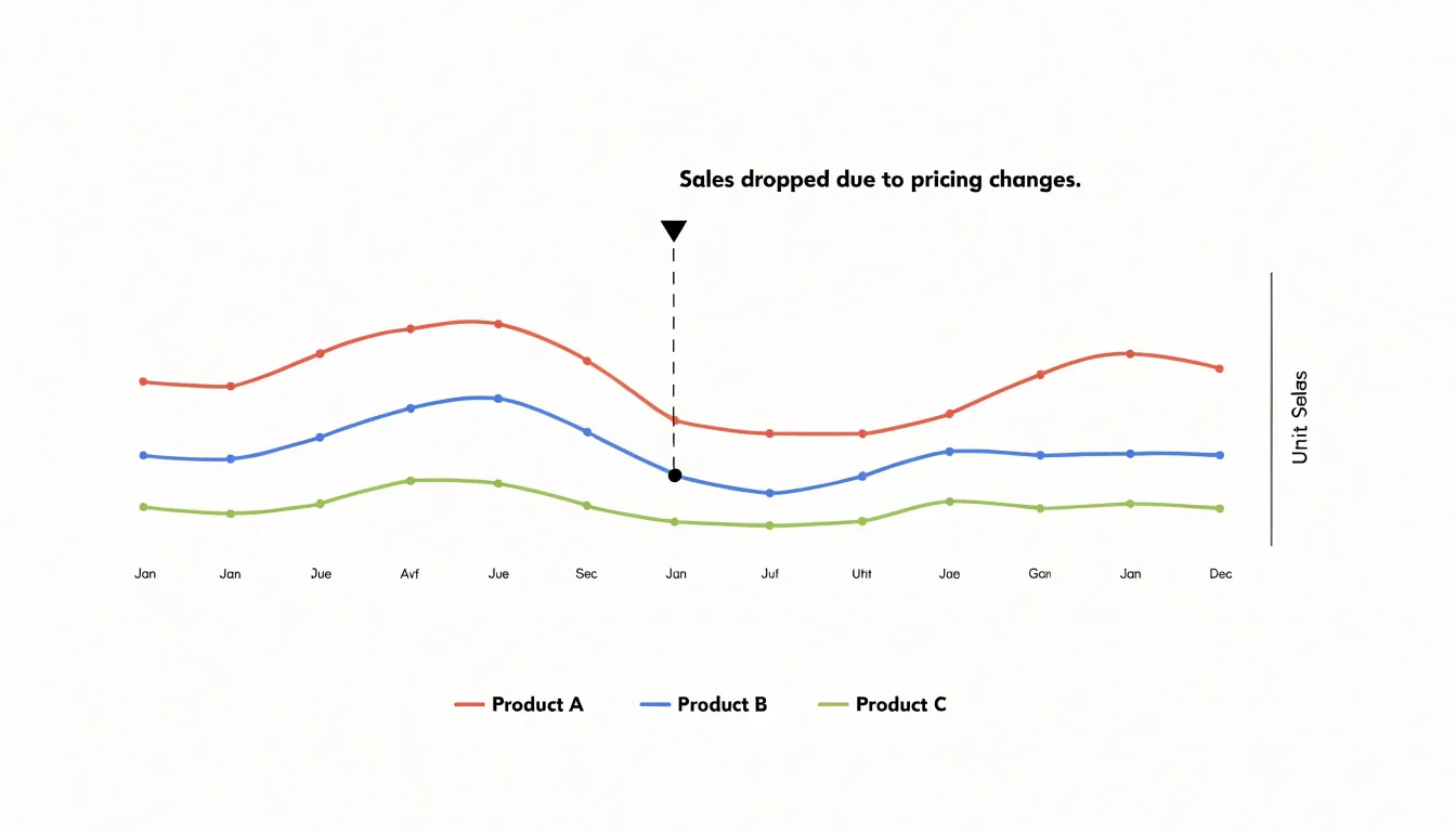
Overlay charts plot multiple series on a single axis, combining line or bar series onto one shared coordinate system. This design lets viewers compare values directly because all series reference the same scale, making intersections and relative positions immediately visible. When two lines cross, for example, the point of intersection shows exactly where the series are equal, and the shared axis allows precise reading of values at that point. The same principle applies to bar series: overlapping or grouped bars on a common axis reveal differences in magnitude without requiring mental conversion between separate scales. The primary advantage of overlay charts is their ability to highlight direct intersections and exact relationships. Because all series share the same x and y axes, viewers can quickly identify where one series overtakes another, where they converge or diverge, and how gaps between them change across the domain. This makes overlay charts particularly effective for showing correlations, competitive trends, or any scenario where the relative position of series is the key insight. For instance, a line chart with multiple series can show how different products’ sales track each other over time, with intersections marking points of equal sales. The shared axis also supports consistent visual encoding: colors or line styles distinguish series, while the common scale grounds all comparisons. However, overlay charts work best when the number of series is limited and the data ranges are compatible; too many series or vastly different scales can clutter the view and obscure the very relationships the chart aims to reveal. When used appropriately, overlay charts provide a compact, direct way to compare multiple series and expose exact relationships at a glance.
Trend Comparison
When the analytical goal is to follow how several series evolve across time, small multiples offer a distinct advantage through their layout of side-by-side panels sharing identical axes. Each panel presents one series against the same temporal scale, allowing the eye to read the shape of every trajectory independently. A reader can trace a gradual upward drift in one panel while noticing a flattening or a late reversal in the adjacent one, without the visual noise that comes from lines crossing and overlapping. Subtle differences in slope, inflection points, and the timing of gradual changes become legible because each series occupies its own space. This matters when the shifts are small in magnitude yet meaningful in direction, since a gentle divergence that would be buried under denser lines in a single frame stands out clearly when isolated in its own small chart.
Overlay charts address a different question. When the interest lies in synchronized movement, a shared plot makes alignment immediately visible. Peaks and troughs stacked on one set of axes let the viewer see which series rises or falls at the same moment, and how far apart their extremes sit. Coincident movements, simultaneous turning points, and the relative height of shared events are read at a glance because the series are drawn against one another rather than separated. The strength of the overlay is this direct, positional comparison of events occurring at the same time, where the question concerns coordination and magnitude at a given moment rather than the private shape of each path.
Choosing between the two comes down to the reader’s task. For independent directional analysis across time, small multiples keep each trajectory clean and comparable. For simultaneous event comparison, an overlay places the series together so their aligned highs and lows can be weighed directly against one another.
Category Comparison
Several practical criteria help determine whether a grouped single chart or a panel grid better serves a multi-variable comparison. The number of categories is the most immediate consideration. When a single chart must accommodate more than roughly four or five categories per variable, the marks begin to crowd one another, colors grow difficult to distinguish, and legends expand to the point of competing with the data for space. A panel grid resolves this crowding by assigning each variable its own frame, so every category keeps a consistent, readable position regardless of how many categories exist.
The complexity of the variables matters just as much. Simple variables with two or three categories, such as a binary outcome tracked across a few conditions, usually fit comfortably into one grouped chart where readers can compare bars or lines directly against a shared axis. As variables gain more categories, or as the shapes of distributions become the point of interest, panels allow each view to be scaled and read on its own terms without the visual interference of neighboring series.
Scale compatibility is another criterion. Grouped charts work best when all variables share a common range, allowing a single axis to serve every series honestly. When variables differ in magnitude, a shared axis flattens the smaller series until their patterns disappear, while independent axes risk misleading comparisons unless the layout makes the difference explicit. Panel grids make per-variable scaling natural and legible, since each frame carries its own axis.
The intended comparison task should guide the final choice. Readers seeking precise differences between categories within one variable tend to do better with grouped marks sharing a baseline, whereas readers scanning for overall patterns across many variables benefit from the consistent structure of a grid. Matching the layout to the dominant question, the number of categories, and the comparability of scales keeps the chart honest and readable.
Information Density
Information density sits at the heart of every charting decision, because every added mark, series, or panel competes for the viewer’s limited attention. When a dataset grows large, the temptation is to squeeze everything into a single frame, and the result is often the spaghettified line chart: dozens of overlapping lines that cross and tangle until individual trajectories become impossible to trace. The alternative extreme carries its own risk, since splitting data into many tiny subplots can shrink each panel below the threshold where patterns, labels, and axes remain legible. Managing density well means treating clarity as a budget that must be spent deliberately.
A practical first strategy is aggregation and filtering. Rather than plotting every raw observation, you can group by meaningful categories, show summary bands, or highlight a small subset of series while rendering the rest in muted gray as context. Layering in this way lets the primary message stand out without discarding the surrounding data. Interactive techniques extend this idea: hover states, brushing, and drill-down panels allow a viewer to reveal detail on demand, so the static view stays calm while the full dataset remains accessible.
Another lever is visual encoding. Careful use of color, line weight, and transparency can reduce perceived clutter even when many marks share the same space. Consistent palettes, restrained labeling, and removing nonessential gridlines and borders all lower the noise floor. Direct labeling of the most important series often works better than a crowded legend.
When partitioning into small multiples, size each panel generously enough to preserve readable axes and recognizable trends, and limit the number of panels per view so the eye can compare without strain. Ordering panels by a meaningful variable, such as magnitude or category, helps viewers scan the grid efficiently. The guiding principle is to add data only when it earns its place, keeping the chart dense with insight rather than dense with ink.
Outlier Detection
Outlier detection in small multiple layouts begins with establishing a visual baseline for what normal looks like in each panel. When a chart is split into a grid of panels, each panel carries its own scale and rhythm, and readers build an implicit sense of the typical range, slope, and volatility for that series. Once that baseline is set, an abnormal spike stands out as a break in the pattern: a sudden vertical jump, a value that sits far above the cluster of neighboring points, or a dip that drops below the floor established by earlier periods. Because panels sit side by side, a reader can scan the grid and spot the one panel whose shape deviates from its siblings, even when the underlying values differ substantially between series.
Techniques for drawing attention to these anomalies usually work by combining a consistent shared reference with a targeted visual cue. A common approach is to apply a uniform y-axis range across all panels where the data permits, so that a spike in one panel is directly comparable to the peaks in the others. Where scales must differ, a faint reference line marking the historical mean or a threshold band gives each panel an internal benchmark against which an unusual value becomes visible. Color provides a second layer: keeping the main series in a neutral tone and rendering flagged points in a saturated accent color isolates the anomaly without disrupting the overall grid.
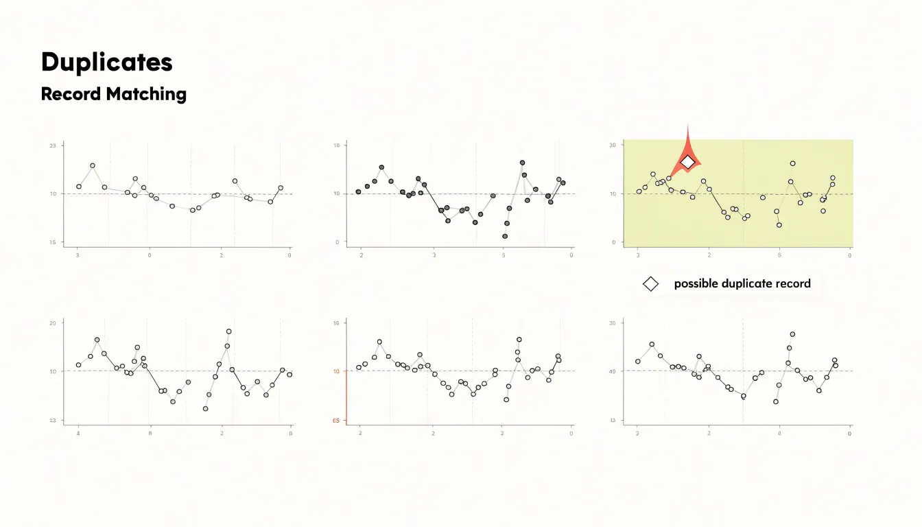
Annotation is the most direct tool. A small label identifying a suspected data entry error, such as a misplaced decimal or a duplicated record, turns a visual oddity into an actionable finding. Automated flagging can be encoded as a distinct marker shape, a hollow circle or diamond, so readers recognize outliers at a glance regardless of color perception. Careful spacing between panels also helps, since generous margins prevent a spike in one panel from visually bleeding into its neighbor and creating a false impression of continuity.
Axis Scaling
When you build a set of small multiples, each panel carries its own y-axis, and that independent axis is where comparison can quietly break down. If one panel’s y-axis stops at 50 and the next panel’s axis stretches to 500, a bar of identical height in both panels represents values that differ by an order of magnitude. The reader’s eye, however, registers equal height as equal magnitude, and the visual message contradicts the data. Maintaining consistent y-axis limits across every panel in the grid keeps the geometry honest: a taller bar means a larger value everywhere in the figure, and the reader can scan across panels with a single mental scale. This consistency is what allows small multiples to function as a comparison tool rather than a collection of unrelated snapshots.
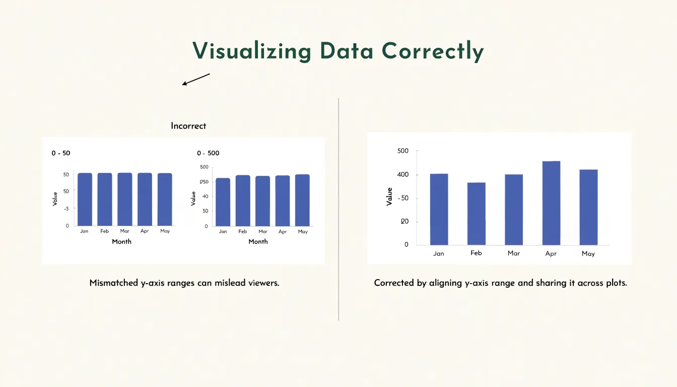
Alignment applies beyond the maximum value. Setting the same minimum and maximum on each y-axis, including the baseline at zero for bar charts, prevents the relative movement of series from being exaggerated or flattened by mismatched framing. When one panel spans a narrow range and another spans a wide one, trends that look dramatic in the first panel may be trivial in the second, and the reader has no visual cue that the scales differ because the panels look identical in every other respect.
Practical implementation often means computing the global minimum and maximum across all series in the dataset and applying those bounds to every panel. Some libraries make this straightforward by accepting a shared domain; others require you to calculate limits manually and pass them in. The slight cost is that individual panels may contain more empty space than they would with fitted axes, but that empty space is a fair price for comparability. In a grid layout, the shared scale is the reader’s anchor, and preserving it protects the integrity of the entire visualization.
Color Usage
Choosing colors for an overlay chart requires a balance between differentiation and harmony. Each series must be distinguishable at a glance, yet the palette should avoid overwhelming the viewer or clashing with established brand guidelines. Start by selecting a limited set of hues—typically no more than five or six—that are perceptually distinct. Use variations in lightness and saturation to create separation, as these differences remain visible even when hues are similar. Tools like ColorBrewer provide research-backed palettes for both categorical and sequential data, ensuring that colors are evenly spaced in perceptual color space. Accessibility is critical: test your palette against common color vision deficiencies (CVD) such as deuteranopia and protanopia. Avoid relying solely on red-green contrasts; instead, combine hue differences with lightness contrasts and consider adding subtle patterns or direct labeling as a backup. Online simulators can help you preview how your chart appears to viewers with CVD. Brand guidelines often dictate primary colors, but for overlay series you may need to extend beyond the core palette. Work within the brand’s secondary colors or create tints and shades of approved hues. If brand colors are too similar, introduce complementary accents from an extended palette that still feels cohesive. Ensure sufficient contrast against the background—especially for thin lines or small markers—by checking contrast ratios (aim for at least 3:1 for graphical elements). Finally, limit visual noise by using muted tones for less important series and reserving vibrant colors for key data. Consistency across charts in the same report helps viewers learn the color mapping quickly. By thoughtfully combining distinct, accessible colors that respect brand identity, you create overlay charts that are both clear and professional.
Cognitive Load
Cognitive load describes the mental effort a viewer spends decoding what a chart presents, and the two designs place that effort in different places. In a shared-axis graph, all series occupy one coordinate space, so the eye moves constantly between lines or marks that overlap, cross, and sometimes occlude one another. Decoding requires holding several visual traces in working memory at once and untangling which segment belongs to which series. The legend becomes a lookup task performed repeatedly, and each glance back to it interrupts the reading of the data itself. Overlapping marks also force the visual system to resolve figure and ground, a process that becomes harder as density increases.
Repeated subplots redistribute this effort. Each small panel contains a single series, so viewers can read any panel in isolation without cross-referencing a legend or separating entangled lines. The cost shifts to scanning: the eye must travel across the grid and compare shapes across space rather than within a single frame. Visual perception research supports the trade-off. Pattern recognition and change detection are faster when a single mark stands alone against a clean background, while comparisons across separated panels rely on spatial memory and saccadic movement between locations. The grid layout also exploits the Gestalt principle of proximity, letting viewers treat each panel as a coherent unit and the whole array as a family of related views.
Working memory plays a central role. Shared-axis charts demand simultaneous retention of multiple series identities, whereas small multiples let viewers compare one panel at a time, keeping the load lower per fixation. The subplot approach trades some precision in direct value comparison for lower perceptual interference, and the shared-axis approach offers immediacy when series counts stay small and separation is clear.
Screen Space
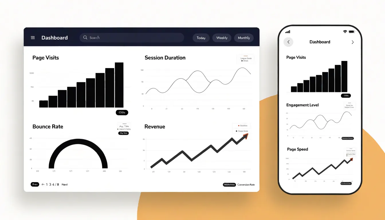
Screen space is the practical constraint that shapes nearly every decision when choosing between overlay charts and small multiples, and it becomes especially acute once a visualization has to survive on both a desktop monitor and a phone. A wide overlay chart assumes generous horizontal room: multiple series share one plotting area, and each additional line, bar group, or marker competes for the same pixels. On a large desktop display this arrangement works well because the chart can stretch across a wide container, the aspect ratio stays comfortable, and viewers can trace individual series without the lines crowding one another. Responsive design for this pattern typically means letting the chart expand to fill its wrapper, adjusting axis tick density, and possibly allowing horizontal scrolling when the series count climbs.
Mobile displays invert those assumptions. A narrow viewport compresses the plotting area, and a wide overlay chart squeezed into that space produces overlapping lines, illegible legends, and axis labels that either collide or vanish. Wrapping a grid layout often solves this problem more gracefully: small multiples can reflow from a single row of panels on desktop into a stacked column on mobile, with each panel keeping a readable aspect ratio and its own compact axis. The grid layout adapts by changing its column count at defined breakpoints, so the same underlying data renders at a workable size regardless of device. Implementing this requires planning container queries or media queries around minimum panel widths, accepting taller page lengths on small screens, and deciding whether to keep a shared legend or repeat labels per panel. The trade-off is vertical scrolling versus visual crowding, and in most mobile contexts the scroll is the friendlier outcome for the reader.
Common Pitfalls
Comparison charts carry a set of recurring failure modes that quietly undermine the very clarity they are meant to deliver. One of the most common is dual-axis misinterpretation. When two series are plotted against separate y-axes, the relative positions of the lines suggest relationships that may not exist in the underlying data. A viewer sees one line cross another and reads meaning into the crossing, even though the two scales are independent and the intersection is an artifact of arbitrary axis ranges. A related habit is truncating the axis, particularly the y-axis, so that it begins above zero. This magnifies small differences into dramatic visual gaps, making modest variation look like a significant trend. The effect is especially misleading when comparing groups whose true values sit close together.
A third pitfall involves cramming too many overlapping series into a single frame. Overlay charts remain readable only while the number of lines or marks stays small. Once a chart holds eight or ten series, the lines tangle, colors repeat, labels crowd, and the viewer loses the ability to trace any individual trend. The result is a dense thicket that conceals the patterns it was built to reveal. Inconsistent color assignment compounds this problem, since the same hue may represent different categories across panels, forcing readers to relearn the encoding each time. Poor labeling and missing legends add further friction. Each of these habits tends to accumulate gradually as charts are revised and reused. Keeping series counts modest, anchoring axes at meaningful baselines, labeling clearly, and reserving dual axes for cases with a genuine shared unit will keep comparison charts honest and legible.
Decision Framework
A decision framework turns chart selection from a matter of taste into a repeatable process. Begin by counting the series you need to display. When a chart carries two or three series, a single overlay chart usually works well because the human eye can track a handful of lines or bars simultaneously. As the count climbs past four or five, overlays grow tangled, colors run out of distinguishable hues, and crossings multiply. At that point small multiples become the stronger choice, since each panel isolates one series and the reader compares shapes across a clean grid rather than untangling a knot.
Next, assess data density. Sparse datasets with a few dozen points per series tolerate overlays without much visual crowding. Dense series, especially those with high volatility or seasonal noise, benefit from the breathing room that faceting provides, because each panel can be scaled and examined on its own terms. Consider also whether the series share a common scale; when magnitudes differ sharply, small multiples with independent axes prevent one dominant series from flattening the rest.
Finally, clarify the primary user goal. If the question is how series relate to one another at specific points in time, an overlay keeps those comparisons direct and immediate. If the question concerns the pattern within each series and how that pattern varies across categories, small multiples support that reading more naturally. Analysts chasing precise value lookups often prefer overlays with tooltips, while audiences scanning for overall shape and outliers do better with faceted panels.
Work through these three checks in order: series count, then density and scale, then the comparison the reader must make. The first branch that clearly favors one format usually settles the decision, and documenting the reasoning keeps future chart choices consistent across a team.
Dashboard Overview
When building executive dashboards, the goal is to deliver clarity and speed. Comparison charts are powerful tools for this, but their integration requires thoughtful design. Start by aligning each chart with a specific decision or question the executive team needs to answer. Avoid clutter by limiting the number of charts to those that directly support key performance indicators. Use small multiples for showing trends across categories, as they allow side-by-side comparison without visual overload. For highlighting differences between two key metrics, overlay charts can be effective when used sparingly and with distinct colors and labels. Ensure consistency in scales and axes across related charts to prevent misinterpretation. Place the most critical comparisons at the top or center of the dashboard, following the natural reading pattern. Incorporate clear titles and annotations that state the insight, not just the data. For example, instead of ‘Sales by Region,’ use ‘Western Region Leads Sales Growth.’ This guides executives to the actionable takeaway. Use color strategically to draw attention to outliers or changes, but avoid overwhelming with too many hues. Interactive elements like filters can help executives drill down, but keep the default view simple. Test the dashboard with actual users to ensure it meets their needs and enables quick comprehension. Finally, ensure that the comparison charts are updated in real-time or at appropriate intervals to maintain trust in the data. By following these best practices, you create dashboards that not only inform but also drive faster, more confident decision-making.
Frequently Asked Questions
What are small multiples?
Small multiples are a series of miniature charts arranged in a uniform grid, with each panel using the same chart type, axis scales, and visual encoding for a different slice of the data. Each metric gets its own dedicated space, so a spike in one series does not hide a dip in another.
When should I use an overlay chart instead of small multiples?
Use an overlay chart when the goal is to show direct intersections and exact relationships, such as where series are equal, overtake one another, converge, or align at the same time. Overlay charts work best when the number of series is limited and the data ranges are compatible.
Why should small multiples share the same y-axis scale?
If one panel’s y-axis stops at 50 and another stretches to 500, bars of identical height represent values that differ by an order of magnitude, while the eye reads equal height as equal magnitude. Consistent y-axis limits, including the same minimum and maximum and a zero baseline for bar charts, keep the geometry honest and let readers scan with a single mental scale.
How many series can an overlay chart show before it gets cluttered?
Two or three series usually work well in a single overlay chart, while overlays grow tangled as the count climbs past four or five. Once a chart holds eight or ten series, the lines tangle, colors repeat, labels crowd, and individual trends become hard to trace.
How can small multiples help detect outliers?
Small multiples help detect outliers by establishing a visual baseline in each panel, so abnormal spikes, dips, or values far from neighboring points stand out. Because panels sit side by side, readers can scan for the one panel whose shape deviates from its siblings, and annotations or accent colors can flag suspected anomalies.
How do small multiples work on mobile screens?
On mobile, a grid of small multiples can reflow from a single row on desktop into a stacked column, with each panel keeping a readable aspect ratio and its own compact axis. This requires planning breakpoints around minimum panel widths and accepting taller page lengths on small screens.
Tony Astor
Tony writes about data visualization and the tools people use to build charts and dashboards. More about Data Illustrator