Small Multiples: Comparing Many Charts at a Glance
 By Tony Astor ·

Small Multiples
Small multiples are a grid of small charts that share identical axes, scales, and color encodings, letting viewers compare many datasets side by side. Consistent scales and layout let the eye detect differences, trends, and outliers almost instantly, reducing cognitive load. They suit time series, regional comparisons, and dashboards where rapid pattern spotting matters.
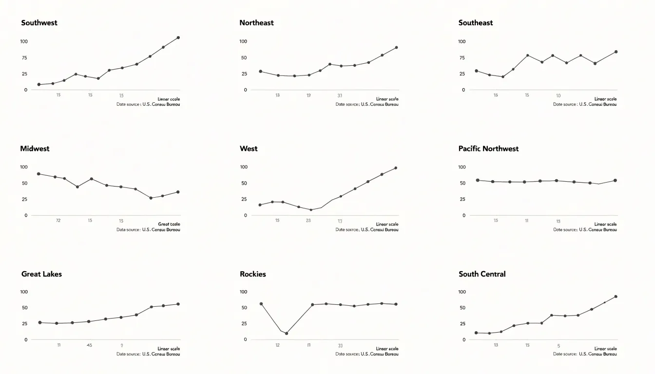
Table of Contents
Small Multiples
Small multiples, or side-by-side charts, derive their power from the way the human visual system is wired. When we look at a series of charts that share the same visual encodings—same axes, same scale, same color palette—our brain can quickly spot differences and patterns without conscious effort. This is because pre-attentive processing automatically detects basic visual features like position, length, and color, allowing us to compare across multiples almost instantly. By standardizing these encodings, we remove the noise of inconsistent designs and let the data speak directly to our perceptual system. The result is a seamless comparison experience: the eye moves from one chart to the next, and variations in the data pop out as salient differences. This leverages our innate ability to detect changes in visual attributes, making small multiples an efficient tool for exploratory analysis and presentation. The consistency across multiples also reduces cognitive load, as viewers don’t need to re-learn the visual grammar for each chart. Instead, they can focus on the data itself, identifying trends, outliers, and clusters with ease.
Design Basics
A grid provides the invisible architecture that holds a set of small multiples together. Before any panel is drawn, the designer decides how many rows and columns the collection will occupy and how each cell relates to its neighbors. Consistent column widths and row heights create a rhythm the eye can follow, allowing viewers to scan across a series and compare panels without recalibrating their attention at every step. When one panel is wider than another or sits slightly off its baseline, the comparison breaks down, and the viewer spends effort decoding the layout rather than reading the data.
Whitespace deserves the same deliberate treatment as the panels themselves. The gaps between cells function as visual punctuation, separating one frame from the next while signaling that all panels belong to a single family. Uniform gutters keep the sequence legible, and a slightly larger margin around the outer edge of the grid frames the whole composition. Crowding panels together can make small differences hard to distinguish, while excessive spacing can fragment the series into unrelated images. The goal is a steady cadence of panel, gap, panel that repeats predictably from the first cell to the last.
Alignment extends beyond the outer edges of each panel. Axis labels, titles, and annotation text should occupy consistent positions within every cell, so that the reader’s eye finds the same information in the same place each time. Shared scales and matched tick marks reinforce this harmony, since a value plotted at the same height in two panels should mean the same thing. When these internal elements drift from panel to panel, the grid loses its coordinating power.
Trend Spotting
Finding patterns across dozens of charts at once requires techniques that make the macro-level structure visible without losing access to the individual panels. One common approach is to scale all panels consistently and order them deliberately, whether by a meaningful variable like region or time period or by a ranking that surfaces clusters and gradations. When panels are ordered by value, a gradient in one direction becomes immediately legible, and any panel that breaks the sequence stands out as a candidate anomaly. Color serves a similar function: assigning a shared color scale across all panels lets viewers scan for the darkest or lightest cells and spot outliers in seconds, while a categorical highlight color reserved for one condition makes correlations between that condition and specific outcomes easy to trace.
Reference elements help here as well; a faint median line drawn identically on every panel gives viewers a fixed benchmark, so panels that sit mostly above or below it read as systematic deviations rather than noise. Small sparklines or marginal summaries within each panel can compress trend information into a consistent glyph, making side-by-side comparison faster.
Finally, annotation plays a role at the macro level. Flagging the handful of panels where an anomaly occurs, or drawing attention to a subset that shares a common pattern, guides the reader’s eye toward the story without requiring a close reading of every chart. The goal is to design the collection so that the pattern emerges from the arrangement itself, letting the reader move from the overview to the specific panel that explains it.
Axis Consistency
Axis consistency means every panel in a small multiple grid uses the same scale on both the X and Y axes, so that a data point in one chart occupies the same visual position it would occupy in any other. When scales are synchronized, a viewer’s eye can compare panels directly: a bar that looks twice as tall genuinely represents a value twice as large, and a line that rises more steeply reflects a faster change. When scales drift apart, the grid becomes a collection of unrelated pictures that invite false comparisons. A panel with a compressed Y axis can make a modest increase look dramatic, while a neighboring panel with a stretched axis can make a large increase look flat. Readers rarely check axis labels panel by panel; they absorb the shapes and carry impressions away with them. Uniform scales protect against that misreading and turn the grid into a single, coherent visual argument.
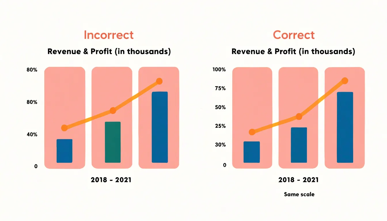
Outliers create the main tension. A single extreme value can force the shared axis to stretch so far that all the ordinary variation collapses into a thin band near the baseline, and the grid loses its ability to show meaningful differences. Several practical options exist. One is to keep the common scale but apply a transformation such as a logarithmic axis, which compresses the extreme value while preserving comparability across panels. Another is to clip the axis at a defined threshold and mark the affected points explicitly, noting the clipping in a caption so no one mistakes a truncated bar for a true value. A third is to reserve a separate detail panel for the outlier while keeping the main grid on a consistent scale. When a full shared range is unavoidable, annotate the extreme panel clearly and use a consistent visual cue, such as an arrow or a broken-axis symbol, so the reader understands that the scale extends beyond what is drawn. The goal is transparency: the reader should never need to guess whether two panels share a common measurement foundation.
Chart Types
Selecting the right core visualization mark begins with a clear understanding of the data’s structure and the question the chart is meant to answer. Line graphs serve time-series data particularly well, because the connected path between points communicates continuity and direction. When observations arrive in a regular sequence—daily sales, monthly temperatures, quarterly revenue—a line lets readers trace the trajectory of a single measure and compare several series over the same horizon. The connecting line implies an ordered progression from one period to the next, so it suits continuous change rather than unrelated categories.
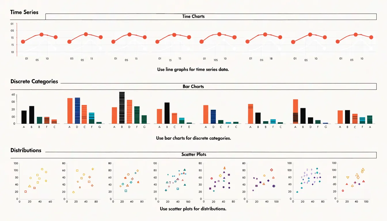
Bar charts handle discrete metrics with a different logic. Each bar represents a separate entity or category, and its length encodes a quantity that readers can compare at a glance. This makes bars ideal for counts, totals, and rankings: the number of support tickets per team, revenue by product line, population by region. Because bars rest on a common baseline, differences in magnitude are easy to judge, and categorical labels sit naturally along the axis. Grouped or stacked variants extend the approach when several measures share the same categories.
Scatter plots address a distinct analytical need: showing how two or more variables distribute and relate across many observations. Each point marks one record positioned by its values on the horizontal and vertical axes, revealing clusters, outliers, and the shape of any association. Scatter plots work best when the underlying data is a collection of individual cases rather than an ordered sequence—customer age against spending, height against weight, advertising spend against conversions. Adding a third variable through color or size turns the scatter into a compact picture of a multivariate distribution.
The choice among these marks should follow the analytical intent. Reach for lines to show change over time, bars to compare discrete quantities, and scatter plots to expose relationships and distributions across individual observations.
Color Strategy
The most effective color approach for small multiples begins with a restrained palette built from a single hue or a narrow range of closely related hues. Using one base color across all panels establishes a consistent visual field, so the eye settles into reading the shape of the data rather than decoding a legend. Varying lightness or saturation within that base hue adds a subtle layer of differentiation between panels while keeping the overall composition calm. A grayscale or muted blue scheme is often sufficient because it lets structural features such as trends, clusters, and outliers emerge on their own.
Selective highlight colors then serve as a spotlight. Once the neutral foundation is in place, a single saturated accent can draw attention to the specific data points, series, or panels that carry the main message. A warm orange or red against a cool gray background creates an immediate focal point, guiding the viewer’s gaze precisely where interpretation matters most. The key discipline is scarcity: limiting highlights to one or two elements at a time. When every panel contains an accent color, the effect collapses and the viewer is back to scanning noise.
Restraint also means resisting decorative variation. Gradients, multiple competing hues, and arbitrary categorical colors multiply the visual load and slow comprehension. Color becomes a quiet instrument of hierarchy rather than an ornament, directing attention toward the story the data is telling.
Labeling
Clear panel titles serve as the entry point for each small multiple, guiding the reader through the comparison. A strong title is concise and descriptive, placed consistently across all panels. Use a consistent format, such as a short noun phrase or a question, to help readers quickly grasp the variable being shown. Position titles at the top of each panel, aligned to the left or center, and maintain uniform font size and style. Avoid overly long titles that clutter the visual; instead, rely on direct data labeling to convey specific values. When possible, incorporate the unit of measurement into the title or axis to reduce redundancy.
Direct data labeling involves placing labels close to the data points they describe, eliminating the need for a separate legend. In small multiples, this approach is particularly effective because each panel can have its own labels without overwhelming the viewer. For line charts, label the end of each line directly with the series name. For bar charts, place value labels at the end of bars. This reduces the cognitive load of matching colors or patterns across a legend and makes each panel self-contained. Ensure labels are legible and do not overlap; adjust positioning or use leader lines if necessary.
Minimalist axis tags further streamline the visual by removing redundant text. In a grid of small multiples, shared axes can be labeled once, typically on the left column for the y-axis and the bottom row for the x-axis. This avoids repeating axis titles and tick labels in every panel. For axes that vary across panels, include only essential tags, such as the variable name and unit, and use short forms where possible.
Sorting Panels
Once the layout of a small multiples grid has been settled, the next decision concerns sequence. Sorting panels determines which chart the viewer encounters first, which sits at the center, and which waits at the corner. This ordering is rarely neutral; every arrangement implies a judgment about what matters and invites the eye to draw comparisons in a particular direction. A deliberate sort turns a collection of independent charts into a coherent narrative, while an arbitrary one leaves the viewer to do the interpretive work alone.
Ordering by magnitude is the most direct method. Panels are ranked by the value of their key measure—such as lowest to highest mean, total, or slope—so the largest values appear at the top left where scanning typically begins. This arrangement creates a visual ranking that surfaces extremes and natural breaks immediately without requiring readers to consult every cell. Alphabetical ordering serves a different purpose: it provides a stable, predictable structure that helps viewers locate a specific category quickly, which is valuable when the grid contains many entities and the audience is likely to search for a particular one rather than absorb the whole picture at once.
Custom narrative logic goes further, grouping panels by shared characteristics such as region, trend direction, or stage in a process. A sequence might move from best to worst performance, from earliest to latest period, or from baseline to outlier. Such ordering encodes an argument about relationships and rewards a reader who follows the grid in the intended order. Whichever method is chosen, the sort should be stated explicitly, whether through labels, a brief caption, or an on-page note, so viewers understand the principle behind the sequence and can interpret the comparison correctly.
Decluttering
In a small multiples layout, each panel inherits the visual furniture of the whole composition, so every redundant element gets multiplied by the number of frames on the page. A legend repeated beside each chart, a set of heavy gridlines redrawn in every cell, or axis labels restated for each row of panels all accumulate into a dense texture of marks that competes with the data itself. Decluttering begins with an audit of what each element contributes. A shared legend placed once at the top of the grid can serve every panel, freeing each frame to carry only its own plotted values. Gridlines can be thinned, lightened, or removed entirely where the data shapes already communicate scale, and tick marks can shrink to short, unobtrusive strokes. Relying on the regularity of the grid allows outer-edge axis labels to imply that the scale repeats across rows and columns.
The guiding principle is the data-ink ratio: the proportion of ink devoted to actual data values versus ink spent on decoration, framing, and repeated scaffolding. In a single chart, trimming excess ink yields modest gains. Across a repeating layout, those gains compound, because the same cleanup applies to every panel simultaneously. Stripping away the noise sharpens comparison, since viewers can scan across panels without their attention caught on borders or restated labels. Decluttering is therefore a structural decision as much as an aesthetic one, shaping how easily a reader moves from one small chart to the next.
Time Series
Time series data often involves multiple groups—demographic segments, geographic regions, or product categories—each with its own trajectory over time. Plotting all these lines on a single chart can quickly lead to a tangled mess of overlapping lines, making it difficult to discern individual patterns and compare trends. Small multiple line charts solve this by giving each group its own mini-chart, arranged in a grid. This layout allows viewers to track temporal patterns across groups without the clutter of overlapping lines.
For example, if you are analyzing monthly sales across different product categories, a small multiple for each category would show its seasonal peaks and troughs. You can quickly scan the grid to see which categories are growing, which are declining, and which have similar seasonal patterns. Because the panels share axes, the visual comparison remains fair, and a large number of groups can be displayed without a complex legend. Isolating each trajectory in a coherent grid also makes it easy to spot temporal outliers in specific groups.
Geographic Grids
Geographic grids offer a powerful alternative to conventional maps when the goal is to compare regional metrics across many locations at once. In a standard choropleth map, the visual weight of each region is tied to its land area, so large but sparsely populated territories dominate the viewer’s attention while small but densely populated ones shrink into insignificance. A grid-based arrangement solves this by giving every region an equal-sized cell, typically a square or tile, positioned in a layout that roughly mirrors the geography of the underlying area. The result is a schematic that preserves spatial intuition—viewers can still locate the Northeast in the upper right or the Midwest in the center—while ensuring that each region’s visual footprint matches its analytical importance rather than its physical size.
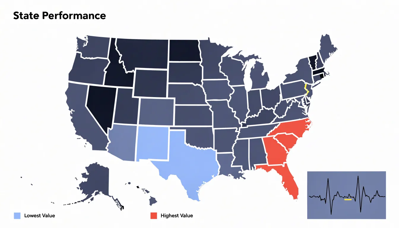
This equal-area treatment is especially valuable when the metric being displayed varies independently of land mass. Population density, electoral results, public health indicators, and economic output all tend to concentrate in small, urbanized regions that a traditional map renders nearly invisible. By allocating one tile per region, grid maps let small states or provinces carry the same visual weight as larger neighbors, making regional differences far easier to perceive and compare. The uniform cell size also supports consistent encoding of color, size, or symbols within each tile, so patterns such as clusters of high values or gradual transitions across neighboring regions emerge clearly.
Tile-based panels extend this logic into small multiples, where each tile in the grid becomes its own miniature chart. Rather than filling a cell with a single color, each region can display a sparkline, bar, or symbol encoding its own time series or distribution. This arrangement combines the geographic anchoring of the grid with the comparative power of small multiples, allowing readers to scan across dozens of regions and spot both local anomalies and broader regional trends. The approach works particularly well for dashboards and reports where space is limited and the audience needs to absorb many regional comparisons quickly.
Layout Mistakes
Layout problems in small multiples tend to compound quietly. Because each panel looks reasonable on its own, the collection as a whole can drift into inconsistency without an obvious culprit. Unequal aspect ratios are a frequent offender. When one panel is taller or wider than its neighbors, the eye reads the difference as meaningful, even when it is purely an artifact of how the chart was sized. Fix this by locking every panel to the same width and height, then letting the grid, rather than individual charts, determine overall dimensions. A shared aspect ratio also keeps trends visually comparable across rows and columns.
Independent Y-axis scaling is another subtle trap. If each panel computes its own minimum and maximum, the collection exaggerates minor fluctuations in some panels and flattens large swings in others. The fix is to compute the axis domain once across the full dataset and apply it to every panel, using a shared log scale or explicit domain annotations when values differ by orders of magnitude.
Cramped padding deserves equal attention. Panels pressed against one another blur the boundary between datasets, and titles or tick labels can collide with neighboring charts. Give each panel breathing room through consistent internal margins, then add deliberate space between panels so each reads as a distinct unit. A final pass with a ruler approach, checking gaps, margins, and baseline alignments numerically, catches the small drifts that accumulate during iteration and keeps the whole composition legible.
Mobile Adaptation
Small multiples work well on wide screens where many panels sit side by side, but on mobile viewports this arrangement collapses under its own density. A responsive approach begins by treating the grid as a variable rather than a fixed frame, so the number of columns adjusts to available width and the overall composition degrades gracefully instead of shrinking every panel into illegibility. The most reliable adaptation converts a multi-column grid into a single-column vertical scroll layout, stacking panels one after another so each receives the full width of the screen. This preserves the internal detail of every chart, keeps labels and tick marks readable without zooming, and maintains the shared scale that gives small multiples their comparative value.
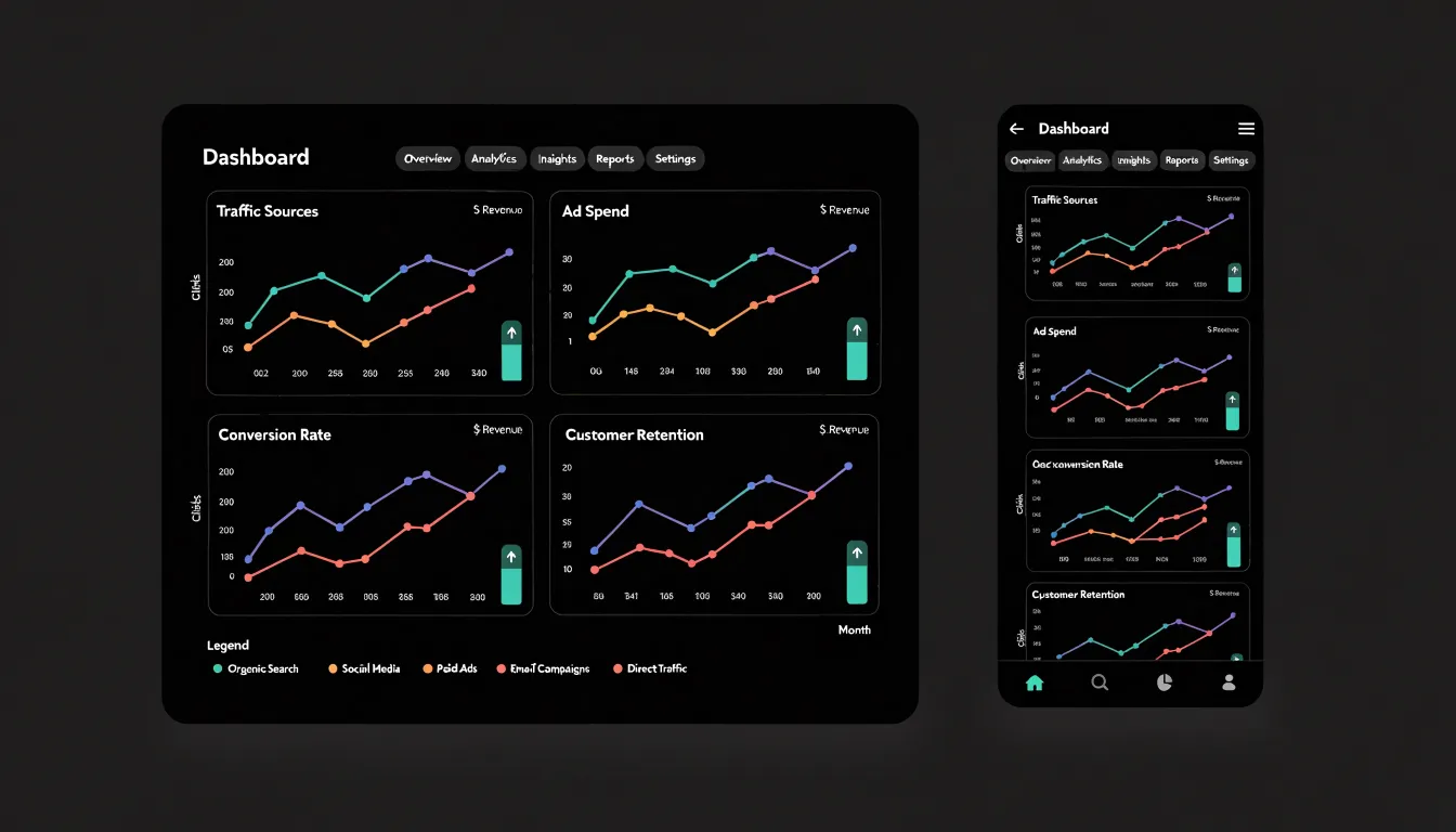
When stacking panels, designers should keep consistent spacing between them, carry over the shared axis and legend so readers do not lose context as they scroll, and consider repeating key reference lines within each panel. Ordering matters as well; arranging stacked panels by the same sequence used in the desktop grid preserves the narrative logic of the comparison. Some layouts benefit from a two-column compromise on mid-sized screens before dropping to a single column, though a simple breakpoint structure is often easier to maintain. Interaction can supplement the scroll: sticky headers, a persistent legend, or a small progress indicator helps readers track position across a long stack. Touch targets should be sized generously, and any tooltips or hover states need equivalent tap behavior. Performance also deserves attention, since loading many panels at once can strain mobile connections; lazy loading panels as they enter the viewport keeps the experience smooth.
Real World Examples
Examining real-world implementations of small multiples offers practical insight into how the technique succeeds across different domains. In financial reporting, annual reports and investor dashboards frequently arrange a grid of sparkline-style charts, each representing a single metric such as revenue, operating margin, or cash flow across consecutive quarters or years. Because every panel shares an identical axis scale, readers can scan the grid and instantly compare volatility and trend direction between business segments without reorienting themselves at each chart. This consistency turns a dense financial summary into a coherent visual narrative that supports rapid executive review.
Scientific publishing has long relied on multi-panel figures to communicate experimental results. Journals in fields such as epidemiology and climate science routinely present a matrix of maps or time-series plots, one panel per region or model run, with a fixed color scale spanning all panels. This design lets reviewers see both the overall pattern and the outliers, while the shared legend prevents the misinterpretation that arises when scales differ between panels. Careful captioning and uniform axis labels make these figures self-contained and reproducible, qualities that peer review demands.
Data journalism provides some of the most accessible examples. Outlets covering elections, public health, or economic inequality often publish grids of small line or bar charts, one per country, state, or demographic group, arranged to invite comparison at a glance. Interactive versions sometimes allow readers to sort or highlight panels, but the underlying principle remains constant: each panel tells a small story, and the arrangement tells the larger one.
Dashboard Overview
Enterprise analytics dashboards serve as the daily entry point for executive teams who need to understand how each department is performing without digging through raw data. In a small multiples dashboard, each panel represents a department, a region, or a product line. A sudden dip in one panel stands out against the steady rhythm of its neighbors, prompting a closer look without requiring the executive to open a separate report or request an analyst’s time. Executives can spot a department whose revenue trend is flattening while others climb, or a region where customer satisfaction is drifting downward, within seconds of opening the dashboard. This rapid high-level visibility supports faster triage and more focused conversations in leadership meetings.
Small multiples also give teams a shared reference point. Because everyone sees the same grid with the same encoding, discussions about performance trends begin from a common visual understanding. A marketing lead and a finance lead can point to the same panel and agree on what the trajectory shows. Over time, repeated exposure to the grid builds pattern recognition across the organization, so anomalies and emerging trends are flagged earlier and escalation happens with better context. The dashboard becomes a lightweight monitoring instrument that keeps departmental performance visible and comparable on an ongoing basis.
Frequently Asked Questions
What are small multiples in data visualization?
Small multiples, also called side-by-side charts, are a series of charts that share the same visual encodings—same axes, same scale, and same color palette—so viewers can compare patterns quickly. The article says this consistency reduces cognitive load and lets pre-attentive processing detect differences in position, length, and color almost instantly.
Why should small multiples use consistent axes?
Axis consistency means every panel uses the same scale on both the X and Y axes, so a data point occupies the same visual position across charts. The article notes that drifting scales invite false comparisons, while uniform scales protect against misreading and make the grid a coherent visual argument.
How should you handle an outlier in a small multiples grid with a shared axis?
The article says a single extreme value can stretch the shared axis and collapse ordinary variation. Options include using a logarithmic axis, clipping the axis at a defined threshold and marking and captioning the clipped points, reserving a separate detail panel for the outlier, or annotating the extreme panel with a consistent visual cue such as an arrow or broken-axis symbol.
When should you use a line chart instead of a bar or scatter plot in small multiples?
Use line graphs for time-series data where connected points communicate continuity and direction, bar charts for discrete quantities like counts, totals, and rankings, and scatter plots for distributions and relationships among individual observations. The choice should follow the analytical intent: lines for change over time, bars for discrete comparisons, and scatter plots for relationships.
What color strategy works best for small multiples?
The article recommends a restrained palette built from a single hue or closely related hues, often grayscale or muted blue, with lightness or saturation variation between panels. Use one saturated accent color sparingly—one or two elements at a time—to spotlight the main message; when every panel has an accent, the effect collapses into noise.
How should small multiples adapt to mobile screens?
A common responsive approach converts a multi-column grid into a single-column vertical scroll, so each panel gets the full screen width and labels remain readable without zooming. The article also says to keep consistent spacing, carry over the shared axis and legend, repeat key reference lines when useful, preserve the desktop ordering, and use generous touch targets with tap equivalents for tooltips or hover states.
Tony Astor
Tony writes about data visualization and the tools people use to build charts and dashboards. More about Data Illustrator