Slope Chart vs Line Chart: When Two Points Are Enough
 By Tony Astor ·
Slope Chart vs Line Chart
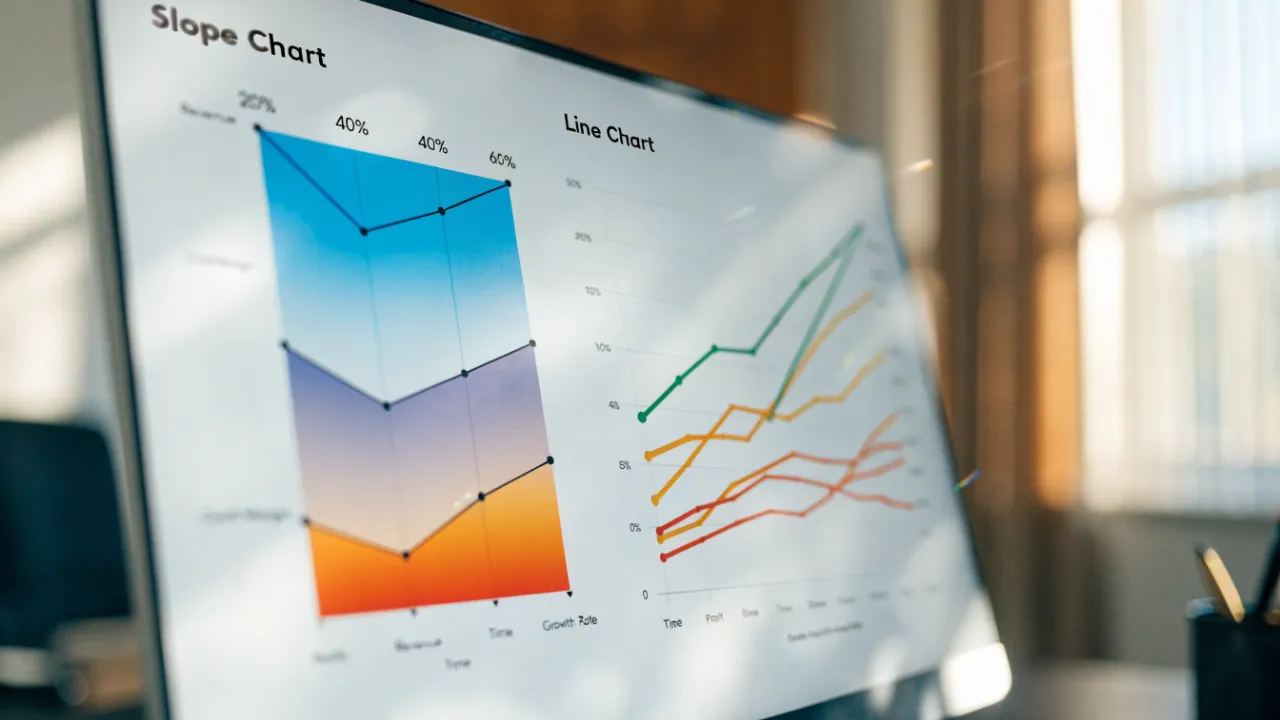
A slope chart compares exactly two points in time, connecting each entity’s start and end values with a straight line so net change reads as a single angle. A line chart connects many consecutive data points with a continuous stroke, revealing trends, fluctuations, and trajectory over time. Use a slope chart for before-and-after comparisons; use a line chart when the path between points matters.
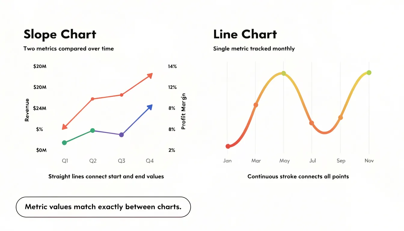
Table of Contents
Line Chart
A line chart connects individual data points with a continuous stroke, and that simple act of connection is what makes it such a strong instrument for reading change across time. When the horizontal axis carries a steady sequence of dates, months, or years, the eye follows the line from left to right and registers motion: a rise here, a dip there, a plateau that stretches across several periods. This continuous path lets viewers perceive the shape of a trend rather than a stack of isolated values, which matters when the underlying data is dense and the story lives in the movement between points.
Fluctuations become legible because the line’s steepness encodes pace. A sharp upward segment signals rapid growth, a gentle slope signals slow drift, and a vertical drop signals an abrupt shock. Readers can compare the relative size of these movements at a glance, spotting spikes and troughs without mentally comparing bar heights or table figures. Seasonality shows up just as naturally. When a series repeats a pattern each year, the line rises and falls in a rhythm that the eye picks up quickly, especially when multiple years are plotted side by side and the recurring peaks align into a recognizable cadence.
Trajectory is where the line chart is most persuasive. The overall direction of the stroke, read from the first point to the last, communicates whether a quantity is climbing, declining, or holding steady. Because the line occupies the full plot area, it uses vertical space efficiently and keeps the reader oriented even when hundreds of points are present. This density tolerance is a real advantage: daily sales, hourly traffic, or monthly revenue can all be plotted without the chart collapsing into clutter, since the connecting stroke smooths the visual noise while preserving the underlying pattern.
Slope Chart
A slope chart is built around the direct comparison of two specific moments in time. The structure is deliberately minimal: a vertical axis on the left represents a baseline period, a vertical axis on the right represents a final period, and a line connects each entity’s value across the two. Reading the chart means tracing a single line from its starting position to its ending position and observing the overall net change between those two anchors. This two-point framing is what defines the mechanics of the slope chart. Each line rises, falls, or holds steady, and the steepness of that line communicates the magnitude of the shift relative to the scale of the axis. Because only two moments are displayed, there are no intermediate fluctuations to interpret. The viewer’s attention stays fixed on the distance traveled between the baseline metric and the final outcome. Entities can be ranked and ordered on both axes so that crossings become meaningful, and a line that crosses others signals a change in relative standing as well as an absolute shift. Color and labeling reinforce which entity performed well and which declined. The result is a compact snapshot of net change across a set of items, suited to cases where the beginning and end of a story matter most. This makes the slope chart especially useful in reporting contexts, where an audience wants to see how a metric like revenue, headcount, or market share moved from one defined point to another, and wants that comparison available at a glance without the noise of every intervening period.
Two Points vs Many
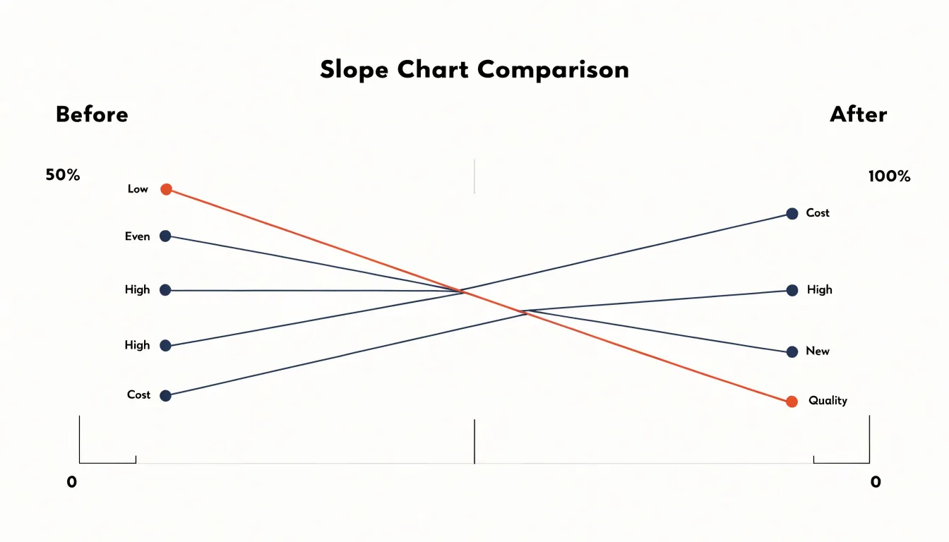
The decision between showing two points and showing many rests on what the audience needs to understand. A two-point display presents a start and an end, which suits situations where the core message is a simple before-and-after comparison: a value was one thing, and now it is another. The reader grasps the change instantly and can hold the entire story in mind without scanning a dense plot. This clarity comes at a cost, because the path between the endpoints disappears, and with it any sense of how the change unfolded over time.
Intermediate points earn their place when the journey matters as much as the destination. A line that rises steadily, dips sharply and recovers, or plateaus for several periods tells a richer story about momentum, volatility, and turning points. Each additional point can supply necessary context: it may reveal when a trend began, whether a shift was sudden or gradual, or how a figure behaved during a specific interval. When those details support the narrative’s argument, including them rewards the reader with a more complete picture.
Noise enters when intermediate points multiply without adding interpretive value. Dense series can bury the headline, slow comprehension, and invite the eye to chase fluctuations that carry no meaning for the point being made. The test is whether each point answers a question the audience is likely to ask. If the reader wonders why a number changed, intermediate data can answer. If the reader only needs to know that it changed, extra points become clutter. Matching the density of the display to the precision of the message keeps the chart focused on the story it exists to tell.
Rank Shifts
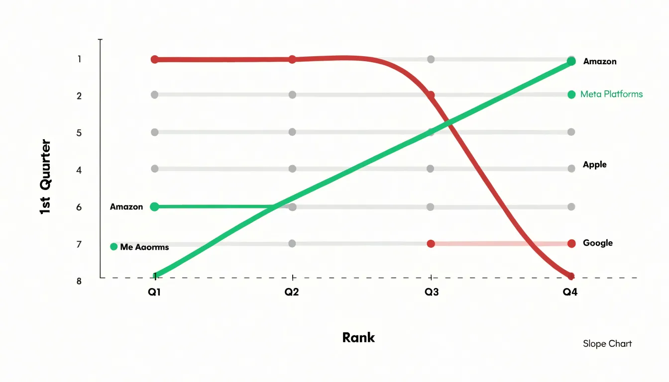
Slope charts excel at revealing rank shifts between two distinct timeframes. By plotting each category’s position on the left axis for the starting period and on the right axis for the ending period, the chart creates a clear visual narrative of how relative standing has changed. The slope of each line directly encodes the magnitude and direction of the shift: a steep upward line indicates a category that has climbed significantly in rank, while a steep downward line signals a sharp decline. Horizontal lines represent categories that have maintained their position. This design makes it easy to spot sudden changes in hierarchy at a glance. For example, in a competitive market analysis, a slope chart can instantly show which companies have overtaken rivals or fallen behind over a year. The limited number of categories—typically no more than 10 to 15—ensures that the chart remains uncluttered and the rank shifts stand out. Additionally, color can be used to group categories or highlight those with notable movements, further drawing attention to the most dramatic changes. The slope chart’s strength lies in its ability to focus on the endpoints of a time period, making it ideal for comparing snapshots rather than continuous trends. When the goal is to communicate how the order of items has changed between two points in time, a slope chart provides a compelling and immediate visual summary that is often more effective than a line chart, which might obscure such rank changes amidst the noise of intermediate fluctuations.
Before and After
Slope charts excel at revealing change between two discrete points in time, making them ideal for before-and-after comparisons. Consider a marketing team evaluating a campaign’s impact on brand awareness across five regions. A slope chart plots each region’s awareness score before the campaign on the left axis and after on the right, connecting the two with a straight line. The steepness of each line immediately shows the magnitude of change, while the direction indicates improvement or decline. Viewers can quickly identify which regions benefited most and which lagged, without the clutter of a full line chart spanning many time points. The clean, minimalist design focuses attention on the delta—the key metric of interest.
Similarly, policy analysts might use a slope chart to assess the effect of a new regulation on compliance rates across industries. Each industry appears as a single line connecting its pre-policy and post-policy compliance percentage. Lines that slope upward signal improved compliance, while downward slopes highlight areas needing attention. The visual simplicity allows stakeholders to grasp the overall pattern at a glance and drill into specific industries as needed. Because slope charts avoid the visual noise of multiple time points, they are particularly effective for communicating a single intervention’s outcomes to diverse audiences.
The key advantage of slope charts in these scenarios is their ability to handle multiple categories without overwhelming the viewer. With a line chart, plotting many categories across numerous time periods can create a tangled web of lines. A slope chart reduces the data to two endpoints, emphasizing the change itself. This clarity makes slope charts a powerful tool for storytelling with data, especially when the goal is to compare the relative impact of an intervention across groups. By focusing on the before-and-after state, slope charts help decision-makers quickly see what worked and what didn’t, facilitating more informed actions.
Removing Clutter
Removing clutter is one of the most effective ways to keep a slope chart focused on the key data. Gridlines are a common source of visual noise, and in most slope charts they can be reduced to a single horizontal line at the starting value or removed entirely, since the two vertical axes already anchor the reader’s sense of scale. When gridlines remain, making them light gray and thin ensures they sit behind the data rather than competing with it. Labels deserve similar scrutiny: endpoint values on the left and right axes are essential, but intermediate tick labels often add little and can be dropped once the axes are clearly marked. Series names can be placed directly at the start or end of each line instead of in a separate legend, which eliminates the eye travel that a detached legend requires. Decorative elements such as drop shadows, background fills, heavy borders, and rounded corners around the chart area all draw attention away from the slopes themselves and can be stripped away without any loss of meaning. Color should carry information rather than decoration; highlighting only the two or three lines with the most significant shifts in a strong hue while rendering the remainder in a muted gray creates an immediate visual hierarchy. The same principle applies to markers: dots at the endpoints help identify start and end values, while markers along the line are rarely needed. The overall goal is a chart where the steepest and flattest slopes stand out at a glance, and every remaining element earns its place by helping the reader compare changes between the two points in time.
Managing Multiple Items
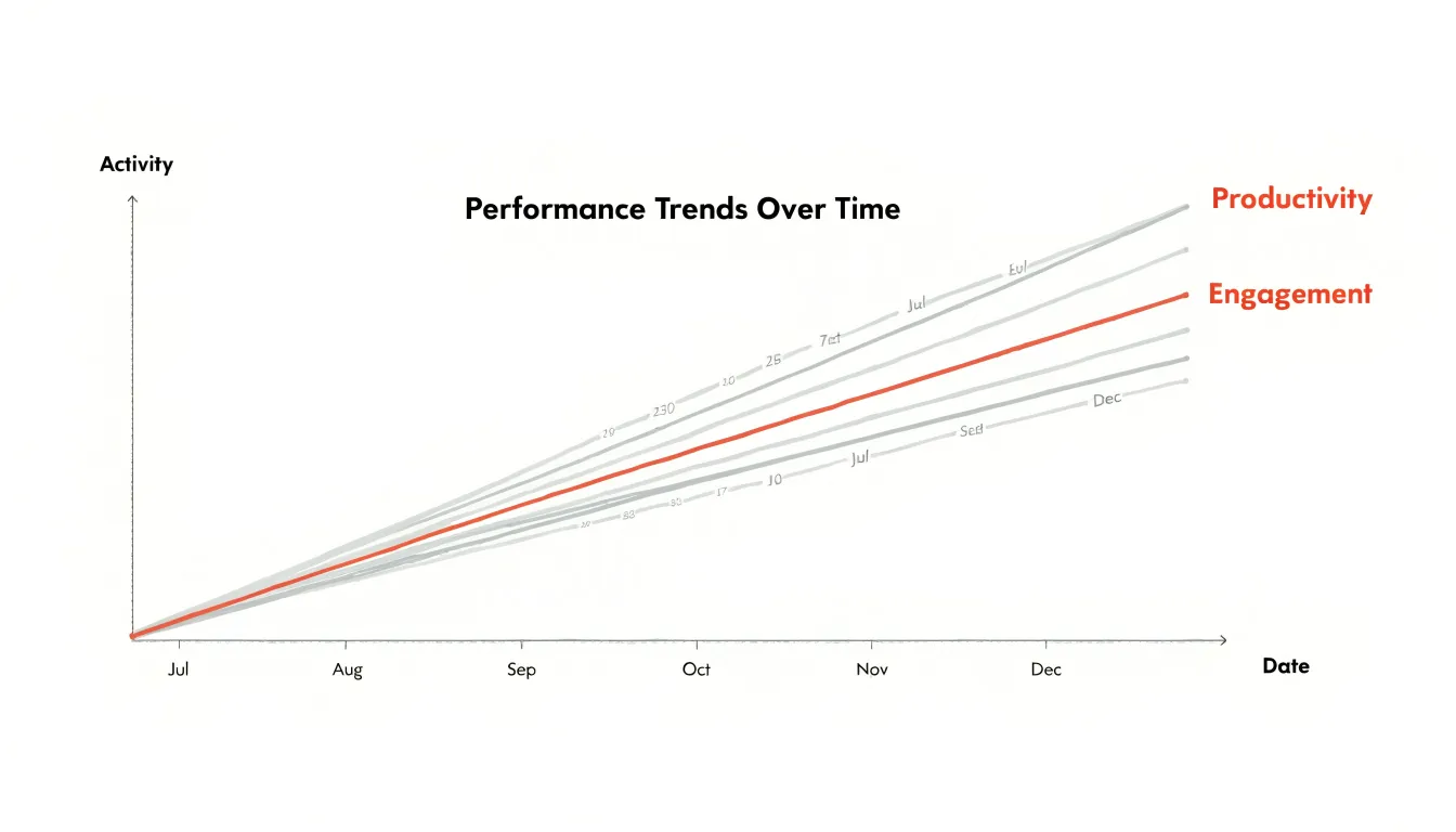
When a slope chart or line chart carries more than a handful of categories, the plotting area can quickly fill with crossing lines until the graphic reads as a tangle rather than a message. The practical remedy is deliberate visual hierarchy. Rather than giving every series equal weight, you assign prominence to the items that carry the story and push the remainder into the background. A common approach is to render the key performers in a saturated accent color while drawing secondary lines in a muted gray or a pale tint of the same hue. The eye then lands immediately on the series that matter, while the faint lines still provide context and comparison without competing for attention.
This technique works because human perception separates foreground from background automatically when contrast is uneven. Viewers do not need to consciously filter the grayed lines; their attention is drawn to the bright ones while peripheral vision registers the rest. The result keeps the chart readable even when it holds fifteen or twenty categories, since the number of visually dominant elements stays small.
Supporting tactics reinforce the same principle. You can vary line thickness, reserving heavier strokes for highlighted series and thinner ones for the rest. Direct labels placed at the ends of lines reduce dependence on a crowded legend and let readers match names to lines without scanning back and forth. Ordering the categories, for instance by final value, helps prevent unnecessary crossings. Interactive treatments extend the idea further, dimming all but the hovered or selected line so that the reader controls which series steps forward.
The underlying discipline is deciding, before drawing, which items deserve emphasis and which serve as supporting cast. That decision transforms a busy chart into a focused one.
Axis and Scale Choices
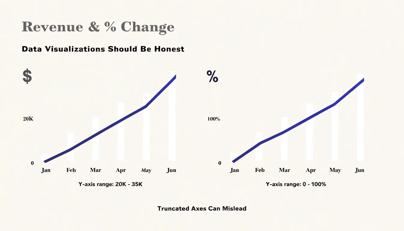
Axis and scale choices determine whether a slope chart or a line chart communicates an honest picture of change over time. The vertical baseline sets the reference point against which every movement is read. Truncating the Y-axis to emphasize small shifts magnifies differences that are modest in absolute terms, so a two-point gain can appear as a dramatic climb. Extending the baseline down to zero tells a more measured story, particularly for values that accumulate from nothing, such as revenue totals or user counts. The appropriate choice depends on the data’s natural range and the interpretive intent, yet the decision should be made deliberately and disclosed to the reader rather than left to whatever default the software supplies.
Proportional spacing matters just as much along the horizontal dimension. When intervals between years, decades, or reporting periods are rendered at equal widths regardless of their true duration, the visual slope no longer corresponds to a real rate of change. A gap of two months placed beside a gap of two years suggests comparable periods of movement when the underlying timelines are wildly different. Placing points at distances that match elapsed time keeps the geometry aligned with the data, so steeper segments genuinely reflect faster change.
Consistent Y-axis scales across panels or small multiples complete the picture. If one facet uses a range of 0 to 100 while another uses 0 to 500, viewers comparing them will misjudge the magnitude of difference between the series. A shared scale, or at minimum a clearly labeled one, ensures that identical visual displacements represent identical numerical shifts. Together, these three decisions create a framework in which both chart forms convey change faithfully, letting the reader trust that what the eye perceives matches what the numbers say.
Ideal Line Chart Scenarios
Line charts excel when the data represents a continuous progression, such as measurements taken at regular intervals over time. The unbroken line connecting each point emphasizes the flow and direction of change, making it easy to spot trends, cycles, and anomalies. For stock price movements, a line chart can display daily closing prices across months or years, revealing long-term trends and sudden fluctuations. The continuous line helps investors and analysts quickly grasp the overall trajectory and identify periods of volatility. Similarly, website traffic trends benefit from line charts when tracking daily or hourly visitor counts. The line’s continuity shows how traffic ebbs and flows, highlighting peak hours, seasonal patterns, or the impact of marketing campaigns. Monthly financial tracking, such as revenue or expenses, also relies on line charts to present a clear picture of performance over consecutive periods. The connected points allow stakeholders to see growth rates, dips, and recoveries at a glance. In all these scenarios, the granularity of the data—frequent, evenly spaced observations—is preserved, and the line chart’s ability to show continuity makes it the ideal choice. The visual emphasis on the path between points helps viewers understand not just individual values but the overall story of change. When the goal is to communicate trends over time, line charts provide a straightforward and effective solution.
Smart Slope Applications
Executive dashboards often need to answer a simple question at a glance: which metrics are improving and which are deteriorating? Slope charts excel at this task because they encode change as a direct visual angle, allowing viewers to compare the steepness of lines connecting two points in time, such as consecutive quarters. For example, a slope chart displaying quarterly revenue growth across business units immediately highlights the units with the sharpest upward slopes—the quick winners—and those with dramatic downward slopes that may require intervention. The human eye is naturally attuned to detecting differences in line angle, so even a crowded dashboard can communicate relative performance without requiring the viewer to parse numbers or legends. This makes slope charts particularly effective in executive summaries where the goal is to surface outliers and prompt further investigation. By focusing on the change between two discrete periods, slope charts also avoid the visual clutter of multi-period line charts, which can obscure the magnitude of recent shifts. In practice, a well-designed slope chart on an executive dashboard might show the top five gainers and losers in market share or customer satisfaction, using color and labeling sparingly to guide attention. The result is a compact, information-dense graphic that supports rapid decision-making and helps leaders spot trends that might otherwise be buried in tables or detailed reports.
Common Visual Errors
Frequent design mistakes in slope and line charts often stem from cluttered composition and distorted scale. Overcrowded lines accumulate when authors plot too many series, each with similar color weights, so that the chart becomes a thicket of crossing strokes. The fix begins with prioritization: highlight the few series that carry the main argument and render the rest in a muted gray, or split a dense slope chart into small multiples that each show a handful of comparisons. Overlapping text labels create their own confusion, particularly at the endpoints of a slope chart where values cluster together. Placing labels directly beside endpoints works well in sparse charts, but when values collide, staggered label positions, leader lines, or a small endpoint table can separate the text without losing the connection to the mark.
Truncated axes represent a subtler problem. Starting a value axis above zero can make modest changes look dramatic, and on a slope chart this distortion becomes especially visible because the visual angle of each segment carries meaning. A steep slope reads as a rapid change, so an arbitrary axis minimum can inflate the impression of growth or decline. The practical remedy is to disclose the axis range clearly and, where comparison matters, keep a consistent scale across related charts. An alternative is to annotate the actual percentage change beside each line, giving readers a literal measure alongside the visual one.
Readability also depends on restraint. Reducing tick marks, using direct labels instead of a remote legend, and keeping a single accent color for the focal series all help the eye follow the intended story. Whitespace between labels and marks prevents text from colliding with lines. Testing the chart at the size it will actually be viewed, on screen and in print, reveals problems that a large editing canvas hides. These small adjustments preserve the chart’s integrity while making its message immediate and clear.
Color and Contrast Tips
Strategic color palettes give slope and line charts their visual hierarchy, letting a reader grasp the main story within seconds of looking at the graphic. The foundation of this approach is a clear division of labor among colors: a small number of saturated, high-contrast hues carry the key messages, while everything else recedes into neutral greys and pale tints. Positive gains typically receive a warm, confident color such as green or teal, applied to the specific lines or endpoint markers that show upward movement. That color signals improvement at a glance and directs the eye toward the segments a reader should celebrate or investigate. Steep declines call for a contrasting accent, often a strong red or orange, reserved for the sharpest drops so that trouble spots stand out immediately rather than blending into a sea of equally weighted data.
Equally important is muting the baseline data. Reference lines, average series, and background trends should be rendered in light greys, thin strokes, or low-opacity tones so they provide context without competing for attention. This muting creates visual breathing room and makes the highlighted elements feel deliberate rather than accidental.
Consistency matters as much as palette choice. Use the same color to mean the same thing across every chart in a report, and limit the number of accent colors to two or three so the emphasis retains its power. Consider color-blind-friendly combinations, maintaining distinct lightness values between any two colors that sit side by side. Labels, callout dots, and shaded endpoint bands can reinforce the color coding without adding clutter. When executed well, this layered approach lets the reader follow the narrative the data tells: gains highlighted, declines flagged, and the steady background left quietly in place.
Quick Selection Rules
Begin by counting the total number of time points in your dataset, since this single figure shapes most of the decision. When you have only two time points, a slope chart is almost always the stronger choice: it pairs each entity’s start and end values directly, so the viewer reads change as a single angle rather than a path. As the count grows to three or four points, both forms remain viable, and the choice shifts toward what you want to emphasize. Beyond five or six time points, a line chart typically earns its place, because the additional vertices give the trajectory meaning and let readers trace continuity across the series.
Visual density is the second criterion. Estimate how many entities will appear on the chart at once. Slope charts handle a modest number of series gracefully, with labels placed at each end and lines fanning out or converging in a clean, readable field. Once you pass roughly a dozen series, the endpoints crowd each other and labels collide, which is a signal to move to a line chart where overlapping trajectories are expected and readers can follow individual lines across the full span. Consider, too, whether your audience will read the chart on a screen or in print, since tighter space rewards the slope chart’s compactness while generous space favors the line chart’s detail.
Finally, name your core analytical message in a sentence. If the sentence is about magnitude of change between two moments, such as which teams gained the most ground, the slope chart delivers that comparison most directly. If the sentence concerns the shape of movement over time, such as a gradual rise, a plateau, or a reversal, the line chart carries that story through its connected path. Use this three-part check in order and let the first criterion that clearly favors one form settle the decision.
Final Chart Checklist
Before publishing any chart, run through a structured verification pass that catches problems while they are still cheap to fix. Start with data integrity: confirm that every plotted value traces back to the source dataset, that units and scales are stated explicitly, and that no series was silently dropped during filtering or aggregation. Recompute a handful of points by hand, especially the start and end positions on a slope chart, since anchoring errors there distort the entire story. Next, audit label placement. Every series line needs a label positioned where it cannot collide with neighboring lines or axis text; on crowded slope charts, alternate labels left and right of the endpoints or nudge them vertically until each reads cleanly. Remove labels that duplicate the legend, and make sure numeric annotations sit close enough to their reference points to avoid ambiguity. Contrast deserves its own pass. Check that line colors remain distinguishable for viewers with color vision deficiencies, that gridlines stay visually subordinate to the data, and that text meets a readable size at the dimensions where the chart will actually appear. Test the chart at thumbnail size to catch elements that vanish or blur. Finally, assess message clarity. Ask whether a reader glancing for five seconds would extract the intended takeaway, and whether the title states the insight rather than merely naming the variables. If the chart needs a paragraph of explanation to be understood, simplify the encoding or annotate the key point directly on the canvas. Walk through these four checks in order, document any changes, and view the final rendering on the target medium before publication so the visual delivers its meaning without requiring a guide.
Frequently Asked Questions
When should I use a line chart instead of a slope chart?
Use a line chart when the data represents a continuous progression and the shape of movement over time matters, especially beyond five or six time points. A slope chart is almost always stronger when you have only two time points and want to compare start and end values directly.
What is a slope chart best used for?
A slope chart is best for directly comparing two specific moments in time, such as before-and-after comparisons or start-to-end reporting on metrics like revenue, headcount, or market share. It focuses on the net change between two anchors rather than intermediate fluctuations.
How many categories can a slope chart show?
A slope chart typically stays uncluttered with no more than about 10 to 15 categories; once you pass roughly a dozen series, endpoints can crowd and labels can collide. With deliberate visual hierarchy, a busy chart can still remain readable even when it holds fifteen or twenty categories.
How do I remove clutter from a slope chart?
Reduce gridlines to a single starting-value line or remove them, drop intermediate tick labels once the axes are clearly marked, and place series names at the ends of lines instead of in a separate legend. Also strip decorative shadows, fills, heavy borders, and unnecessary line markers, and use color to highlight only the most significant shifts.
How does a slope chart show rank changes?
A slope chart shows rank changes by plotting each category’s position on the left axis for the starting period and on the right axis for the ending period. Steep upward lines indicate significant rank climbs, steep downward lines signal sharp declines, and horizontal lines represent categories that maintained their position.
What are common visual errors in slope and line charts?
Common visual errors include overcrowded lines, overlapping text labels, and truncated axes. A truncated value axis can make modest changes look dramatic, so the article recommends disclosing the axis range clearly and using a consistent scale where comparison matters.
Tony Astor
Tony writes about data visualization and the tools people use to build charts and dashboards. More about Data Illustrator