Scatter Plot vs Bubble Chart: When to Add Size
 By Tony Astor ·

Scatter Plot vs Bubble Chart
A scatter plot displays two quantitative variables as dots positioned on x and y axes, revealing correlation, trends, clusters, and outliers. A bubble chart extends it by encoding a third quantitative value as marker area, adding magnitude to the same view. Scatter plots suit precise two-variable analysis; bubble charts suit multi-variable comparison where size carries real meaning.
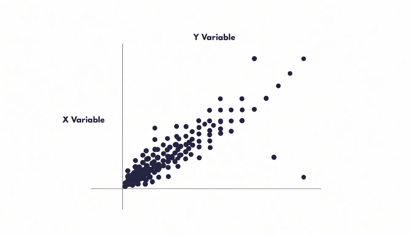
Table of Contents
Scatter Plot
At its core, a scatter plot translates a table of paired values into a field of dots on Cartesian coordinates. One variable is assigned to the horizontal axis and the other to the vertical axis, so every data point lands at the intersection of its two recorded values. When the horizontal variable is treated as the independent quantity and the vertical as the dependent one, the resulting cloud of dots becomes a direct visual statement about how the two measurements move together across the full set of observations.
The real interpretive power of the plot emerges from the shape of that cloud. When points drift from lower-left to upper-right, the distribution signals a positive relationship; when they fall from upper-left to lower-right, the relationship runs negative. The tightness of the pattern matters as much as its direction, since a narrow band of dots suggests a strong association while a loose, sprawling field suggests a weak one. Tracing the overall drift of the dots also makes the general form of the relationship visible, allowing an analyst to judge whether a straight-line summary is reasonable or whether the pattern curves in ways a single correlation coefficient would hide.
Clusters and outliers add further detail. Distinct groupings of dots can point to subpopulations mixed within one dataset, each possibly behaving according to its own rule. Isolated points far from the main mass deserve separate attention, since they may represent data entry errors, unusual cases, or genuinely interesting exceptions that warrant investigation before any modeling begins.
Because the method preserves each individual observation rather than aggregating it, the scatter plot lets trends, groupings, and anomalies be read together in a single view, giving it a foundational place in exploratory analysis.
Bubble Chart
A bubble chart extends the familiar scatter plot by treating the size of each marker as an additional data channel. Where a scatter plot places a point according to two coordinates, a bubble chart attaches a third quantitative value to the physical dimension of that point: its diameter or area. Each marker grows or shrinks in proportion to a metric such as market share, population, revenue, or transaction volume, so a single glance across the plane reveals not only where cases sit relative to one another on the two axes but also how heavily each case weighs on some third measure.
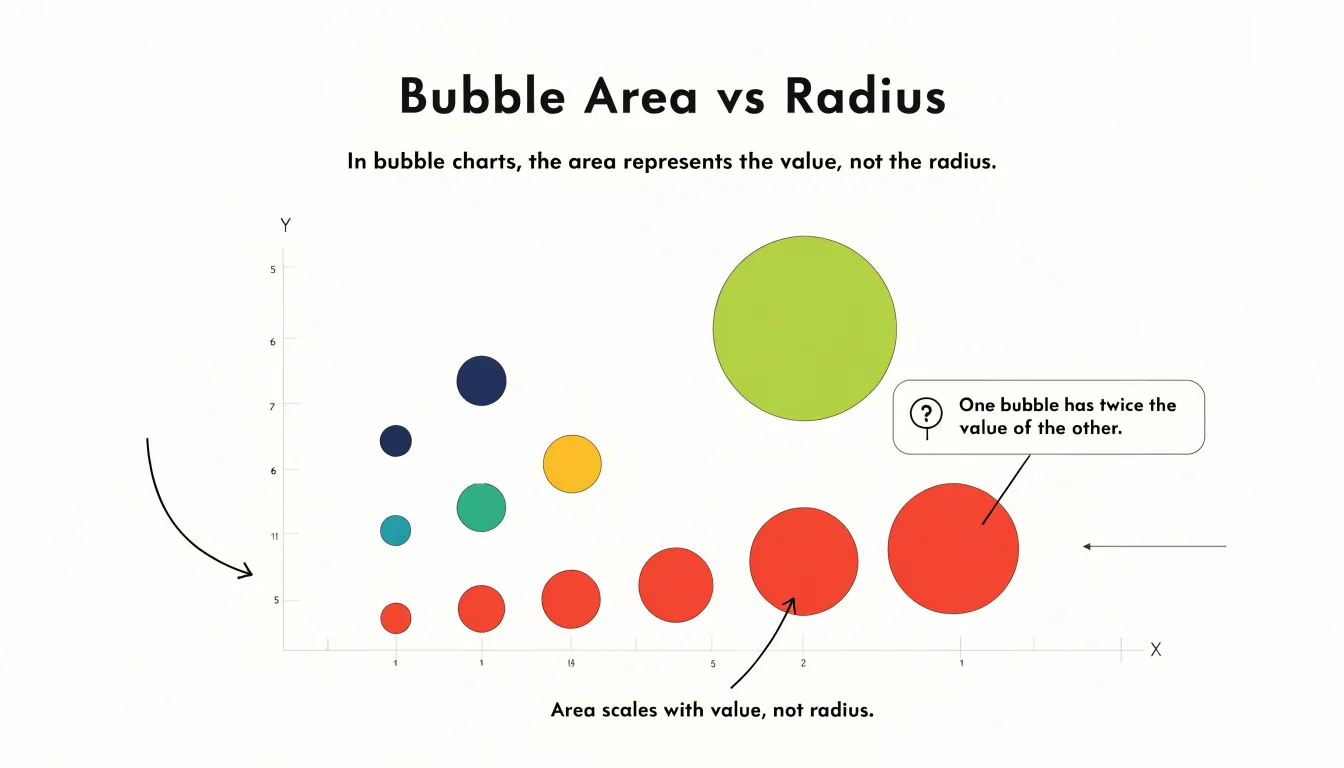
The design value of this expansion lies in the density of information it achieves on a single plane. Analysts can compare many entities at once, watching how position and magnitude interact. A small bubble in the upper-right corner tells a different story from a large one nearby, and clusters of large bubbles signal concentrations of activity that a two-variable chart would leave invisible. Readers can scan for outliers by location, by size, or by the combination of the two, which makes the chart useful for prioritization and segmentation work.
Encoding a third metric through size enriches comparative analysis because it mirrors how decisions are usually made. A product may lead on price and satisfaction while holding a modest share of the market; a bubble chart displays all three facts in one mark. Population against income against land area, or revenue against growth against headcount, can be read in a single view, letting viewers weigh tradeoffs without flipping between charts. The visual expansion keeps the relational strengths of the scatter plot intact while layering magnitude onto the same canvas, so the chart supports richer storytelling and more informed comparison.
Bubble Size
Bubble size is the additional visual channel that distinguishes a bubble chart from a scatter plot, and it carries real quantitative meaning. While position on the horizontal and vertical axes encodes two variables, the diameter or area of each dot encodes a third, letting a single chart communicate three dimensions of data at once. Common examples include population totals on a map, revenue figures across regions, or transaction counts by category. The value assigned to size should be stated plainly in a legend so readers understand what the variable represents and can judge relative magnitudes with confidence. Ambiguity about whether size reflects a count, a sum, or an average undermines the chart’s usefulness.
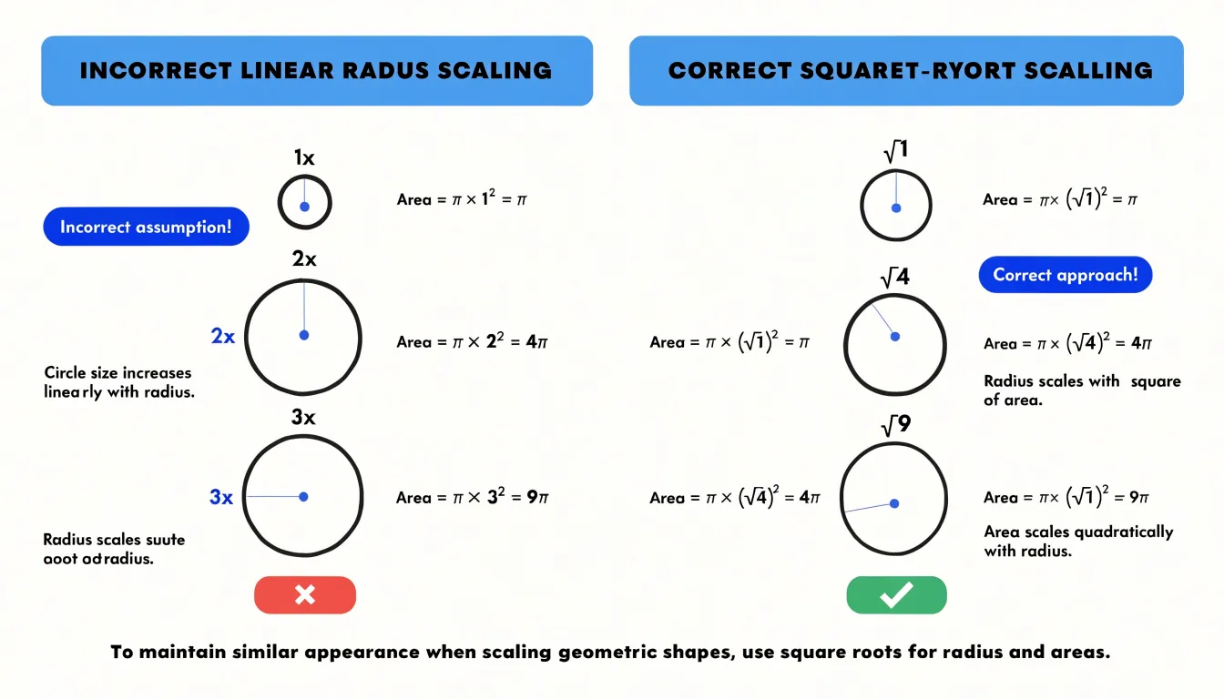
The scaling of that size is where many bubble charts go wrong. Human perception judges the magnitude of a circle by its area, not its diameter. If a designer maps data values directly to radius, a value twice as large produces a circle with four times the area, and the visual impression of difference is exaggerated dramatically. A value three times larger appears nine times heavier on the page. The result is a chart that systematically overstates variation and misleads even careful readers. The correct approach maps data values to area, deriving the radius from the square root of the value. This keeps perceived size proportional to the underlying number and preserves honest comparison across bubbles.
Practical thresholds matter as well. Very small values can produce dots too tiny to see or click, while very large values can swallow neighbors or overflow the plotting region. Setting a sensible minimum size keeps minor categories visible and legible, and a sensible maximum size prevents dominant values from crowding out the rest of the data. Many tools expose these bounds as adjustable parameters, and reviewing them against the actual value range in the dataset is a worthwhile step before publication. Transparent bubbles with a subtle border also help overlapping circles remain readable, since large bubbles will inevitably cover smaller ones in dense regions.
Key Differences
When choosing between a scatter plot and a bubble chart, the most reliable starting point is a feature-by-feature comparison, because each format carries its own strengths and constraints into the analytical task. Begin with dataset complexity. A scatter plot encodes two variables using position along the horizontal and vertical axes, which keeps the visual grammar simple and the decoding process fast. A bubble chart adds a third dimension through the size of each marker, and sometimes a fourth through color. That added encoding allows richer stories, yet every extra channel increases the cognitive load placed on the reader, who must now judge area differences in addition to reading coordinates.
Audience familiarity matters just as much. Position-based charts are among the most widely understood visual forms, appearing in classrooms, news reports, and business dashboards, so viewers can interpret them with little or no guidance. Bubble charts require a legend and a moment of explanation, since readers must learn that size represents a specific quantity and that larger markers may obscure smaller ones. For a general audience or a fast-moving presentation, that learning curve can reduce comprehension.
Visual precision requirements complete the comparison. Judging the area of a circle is considerably harder than judging a point’s distance from an axis, and overlapping bubbles can hide underlying observations. When the task demands accurate reading of correlation strength, slope, outliers, or clusters, the scatter plot preserves precision, which is why analysts favor it for strict correlation work. Bubble charts shine in contextual reporting, where the third variable provides useful background and the goal is to communicate magnitude and relationship at a glance rather than to support exact measurement. Weighing these three features against the purpose of the chart leads to a sound choice.
Visual Clutter
Visual clutter is one of the most common problems that undermines a bubble chart’s usefulness, particularly when the dataset contains many observations packed into a small area. When bubbles are fully opaque and sized generously, they stack on top of one another until individual data points disappear entirely, leaving the viewer with an indistinct mass of color rather than a readable pattern. Adjusting bubble opacity offers a practical first line of defense. Reducing fill transparency lets overlapping regions reveal their density through darker or more saturated color, so clusters become visible as clusters while individual bubbles remain discernible at the edges. A common approach is to pair semi-transparent fills with slightly stronger outlines, which preserves the shape and boundary of each bubble even when interiors blend together.

Responsive scaling addresses the same problem from the dimension of size. If bubble radius is mapped directly and proportionally to a raw value, a few large values can dominate the plot and obscure everything beneath them. Capping the maximum radius, applying a square-root transformation to area, or scaling bubbles relative to the current viewport all keep the visual weight of each mark within reasonable bounds. Responsive scaling also means that as the chart resizes or the visible range changes through filtering, bubble sizes readjust so the plot never becomes denser than the available space can support.
Data thresholds provide a complementary strategy by limiting what appears in the first place. Aggregating tightly packed points into a single representative bubble, filtering out values below a minimum count, or grouping dense regions into summary marks reduces the sheer number of elements competing for attention. Together, these techniques let a bubble chart handle dense or tightly clustered datasets while keeping each mark legible and the overall visualization easy to interpret.
Color and Labels
Color is one of the most efficient channels for encoding a second dimension of information on a scatter or bubble chart, provided it is applied with restraint. When points fall into natural categories such as regions, product lines, or customer segments, assigning a distinct hue to each group lets viewers perceive clusters and separations almost instantly, often before they read a single number on the axes. The eye is remarkably good at detecting similarity and difference in hue, which means categorical grouping through color can replace more cluttered visual cues like varied marker shapes. The key is to keep the palette limited and consistent, since too many hues quickly turn the plot into visual noise.
Labels play a complementary role. Rather than annotating every point, which crowds the canvas and slows reading, strategic labeling focuses attention on the observations that carry the story: the outliers, the extremes, and the handful of cases worth naming. A well-placed label beside a single large bubble gives that data point meaning without demanding that the reader match it against a legend. Used sparingly, labels function as signposts rather than decoration.
Color choices should also stay neutral enough that size stays legible. If hues are highly saturated or strongly contrasting, they can compete with the varying bubble radii and make relative magnitude harder to judge. Muted, harmonious tones allow the diameter of each marker to remain the primary carrier of quantity, while color quietly organizes the categories in the background.
None of this works without an intuitive, clearly positioned legend. A legend that maps each color to its category at a glance lets readers decode the chart without mental effort, so the perceptual gains from color and labeling translate into genuine comprehension.
Common Mistakes
Misleading scales and hard-to-read charts are among the most frequent design pitfalls in scatter and bubble charts. One common mistake is linear radius scaling: when the radius of a bubble is set proportional to the data value, the area—and thus the visual impact—grows with the square of the value. A bubble representing twice the value appears four times larger, exaggerating differences and distorting perception. To correct this, scale the area directly to the value, or use the radius proportional to the square root of the value, ensuring that visual size matches the underlying data. Another frequent issue is poor color contrast. Low-contrast palettes, especially those that do not account for color vision deficiencies, make it difficult to distinguish categories or perceive gradients. Choosing accessible color schemes with sufficient luminance contrast, and avoiding red-green combinations, helps all readers interpret the chart accurately. Overwhelming viewers with too many variables at once is also common—adding size, color, shape, and transparency simultaneously can turn a chart into a confusing mosaic. Limiting the number of encoded variables to two or three, and using clear legends, reduces cognitive load. To spot these mistakes before publication, review the chart at different sizes and on various devices, check that scales are labeled and consistent, and test with a colleague who is unfamiliar with the data. Verifying that bubble areas are proportional to values, that colors are distinguishable in grayscale, and that the chart remains legible when printed or viewed on a small screen are essential final checks. Correcting these issues ensures the chart communicates data faithfully and remains readable for all audiences.
Real World Examples
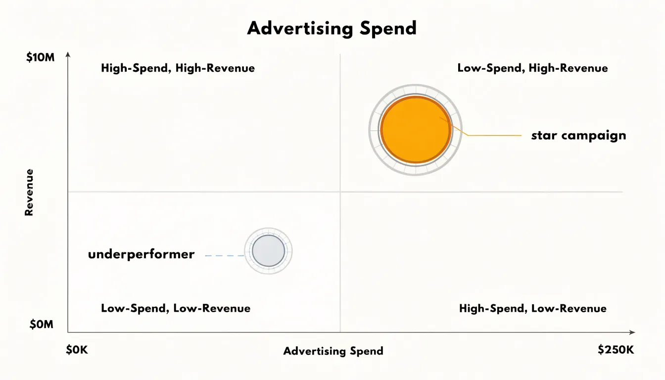
In marketing analytics, scatter plots and bubble charts translate campaign data into clear strategic direction. A scatter plot of monthly advertising spend against revenue, for instance, reveals the relationship between investment and return across different periods or channels. Each point represents a specific timeframe or campaign, allowing analysts to spot positive correlations where increased spend consistently drives revenue growth. Outliers stand out immediately: a campaign with high spend but low revenue signals inefficiency, while low spend paired with high revenue highlights exceptional performance worth replicating. By adding bubble size to represent total customer volume, the visualization gains a third dimension. A large bubble in the high-spend, high-revenue quadrant indicates a campaign that not only generates sales but also acquires many customers, making it a prime candidate for scaling. Conversely, a large bubble in the low-revenue region warns of wasted budget. These layered insights enable executives to allocate resources with precision, focusing on channels that deliver both revenue and customer growth while cutting underperformers. In finance, similar visualizations clarify risk and return profiles. Plotting expected return against volatility for a portfolio of investments, with bubble size reflecting the capital allocated to each asset, helps decision-makers balance risk and reward. Assets with high returns and low volatility appear as small bubbles in the ideal corner, signaling opportunities to increase allocation. Large bubbles in high-volatility areas prompt a review of exposure. Across both domains, the combination of position and size transforms raw numbers into a narrative that executives can act on quickly, fostering data-driven decisions that align with strategic goals.
Cognitive Load
When a scatter plot gains a third dimension through bubble size, the viewer’s cognitive system must simultaneously encode and integrate multiple visual channels. Research on graphical perception shows that position on a common scale is the most accurate channel for quantitative comparison, while size is less precise and more susceptible to systematic underestimation. Adding a size variable therefore introduces a source of error that does not exist in a simple scatter plot. The viewer must also divide attention between the x-axis, y-axis, and the area of each mark, increasing the mental effort required to extract meaning. This extra effort is not inherently negative; it can signal that the data contains richer structure. The trade-off lies in the audience’s capacity to process that structure without losing the main message. For non-technical stakeholders, working memory is limited, and every additional visual attribute competes for attention. If the size variable is central to the story, a bubble chart can work well, provided the legend is clear and the size range is not too extreme. If size is secondary or decorative, it may distract from the primary relationship between x and y. Designers can reduce cognitive load by limiting the number of visual attributes, using consistent scaling, and providing direct labeling where possible. Grouping or filtering can also help viewers focus on one dimension at a time. The goal is to match visual complexity to the audience’s familiarity and the decisions they need to make. A chart that is too simple may omit crucial context, while one that is too complex may be abandoned altogether. Balancing data density with ease of interpretation requires testing the chart with representative users and observing where they struggle. In practice, this means prioritizing the most important comparisons and using additional dimensions only when they add clear value.
Interactive Design
Interactive design transforms a static chart from a fixed snapshot into a dynamic exploratory tool. Hover effects, in particular, allow users to reveal detailed information without overwhelming the initial view. When a user moves their cursor over a data point, a tooltip can display precise values, labels, and even contextual details that would be too cluttered if always visible. This on-demand disclosure keeps the chart clean while still providing access to the underlying data. Zoom functionality further enhances exploration by letting users focus on specific regions of the plot. In a scatter plot with hundreds of points, zooming in reduces visual density and makes individual points easier to distinguish. Similarly, highlight filters enable users to isolate subsets of data by category or value range, temporarily dimming or hiding other points. This reduces visual noise and helps users spot patterns or outliers that might be obscured in a static view. Together, these interactive features mitigate the clutter inherent in static charts, where all information must be presented at once. By shifting detail to user-controlled interactions, the overall aesthetic clarity is preserved, and the chart remains approachable. Users can inspect precise values without sacrificing the big-picture view, making the visualization both informative and visually appealing. Ultimately, interaction empowers users to tailor the view to their needs, enhancing both usability and insight.
Decision Checklist
A decision checklist turns chart selection into a repeatable process, and the first item on that checklist is the number of data points you intend to display. Small datasets with a few dozen marks leave plenty of visual space, so a scatter plot reads clearly and each point stays easy to identify. As the count grows into the hundreds, overlapping marks begin to obscure one another, and the choice of chart type starts to affect whether patterns remain visible. Counting your points before you open the charting tool gives you a realistic sense of how much visual load the final graphic can carry, and it sets the context for every decision that follows.
The second step examines variable types. A scatter plot accommodates two quantitative variables placed on the horizontal and vertical axes. A bubble chart adds a third quantitative variable encoded as the area of each mark, which requires a numeric column with meaningful variation across the dataset. If the candidate third variable is categorical, or if its values cluster so tightly that bubble sizes look nearly identical, size encoding adds little. Confirming that each variable is continuous, complete, and scaled sensibly protects the chart from misleading area comparisons before you commit to it.
The final step connects the data to the story you want to tell. Ask what the viewer should notice first: the relationship between two measures, the position of specific outliers, or the relative magnitude of a third factor. When the third variable carries genuine analytical weight, bubble size earns its place. When it merely decorates the chart, a scatter plot keeps attention on the primary relationship. Working through these steps in order, from point count to variable types to story objective, gives creators a systematic way to validate each design choice and to justify the added complexity of bubble size with a clear analytical purpose.
Dashboard Overview
Executive dashboards succeed when every chart serves the overarching business story. Matching chart choice to that narrative begins with a clear understanding of the story you need to tell. A scatter plot excels at revealing relationships between two continuous variables, making it ideal for questions about correlation, trend, or outlier detection. When a third variable such as market size or revenue impact matters, a bubble chart adds that dimension through size variation. The key is to align the chart’s complexity with the narrative context: a simple two-variable relationship calls for a scatter plot, while a multi-variable comparison that includes magnitude warrants a bubble chart. Integration into executive dashboards requires more than selecting the right chart type; it demands thoughtful placement and design. Place the chart where it supports the flow of the dashboard story, typically after key metrics have set the stage and before detailed breakdowns. Keep the design clean by limiting the number of data points, using clear labels, and ensuring that color and size encoding are intuitive. Overly complex bubble charts can overwhelm executives, so reserve them for situations where the third variable is essential to the decision at hand. Finally, tie the visualization directly to business goals by annotating key insights, such as highlighting target regions or flagging outliers that require attention. This approach ensures that the chart not only displays data but actively contributes to strategic understanding, enabling executives to grasp relationships and make informed decisions quickly.
Frequently Asked Questions
What is the difference between a scatter plot and a bubble chart?
A scatter plot uses horizontal and vertical position to encode two variables, while a bubble chart adds a third quantitative variable through marker size and can sometimes add a fourth through color. This lets a bubble chart show magnitude as well as the relationship between the two axes.
How should I scale bubble sizes in a bubble chart?
Map data values to the area of each bubble, or derive the radius from the square root of the value, so perceived size stays proportional to the underlying number. The article cautions that mapping values directly to radius exaggerates differences because area grows with the square of the value.
How can I reduce visual clutter in a bubble chart?
Use semi-transparent bubble fills with slightly stronger outlines, cap the maximum radius or scale bubbles relative to the viewport, and aggregate, filter, or summarize dense regions to reduce the number of marks competing for attention. These techniques help keep individual bubbles legible in dense or tightly clustered datasets.
What are common mistakes to avoid in scatter and bubble charts?
Avoid linear radius scaling, poor color contrast, and too many encoded variables such as size, color, shape, and transparency all at once. Check scales, test at different sizes and devices, verify bubble areas are proportional to values, and ensure colors are distinguishable in grayscale and avoid red-green combinations.
When should I use a bubble chart instead of a scatter plot?
Use a bubble chart when a third quantitative variable carries genuine analytical weight and you want to communicate magnitude and relationship at a glance. If size would be secondary or decorative, or the audience needs fast, precise reading of correlation, slope, outliers, or clusters, a scatter plot keeps attention on the primary relationship.
How can color and labels improve a scatter or bubble chart?
Use a limited, consistent palette to group natural categories, strategic labels for outliers, extremes, and key cases, and an intuitive, clearly positioned legend. Keep colors muted and neutral enough that bubble size remains the primary carrier of quantity.
Tony Astor
Tony writes about data visualization and the tools people use to build charts and dashboards. More about Data Illustrator