Scatter Plot: How to Show Relationships Between Variables
 By Tony Astor ·

Scatter Plot
A scatter plot is a graph that displays paired data as individual dots on an X-Y coordinate system, with one variable on each axis, so each point represents one observation. It reveals whether two variables are related—showing positive trends, negative trends, no correlation, or non-linear patterns—and how strong that relationship is.
Table of Contents
Scatter Plot Basics
A scatter plot is built on a coordinate system where each axis represents one variable. The horizontal X-axis typically carries the independent variable—the quantity you control, observe, or use as a reference. The vertical Y-axis usually carries the dependent variable—the quantity you measure or expect to respond as the independent variable changes. Deciding which variable belongs on which axis is the first step in constructing the plot and shapes how a viewer interprets the relationship.
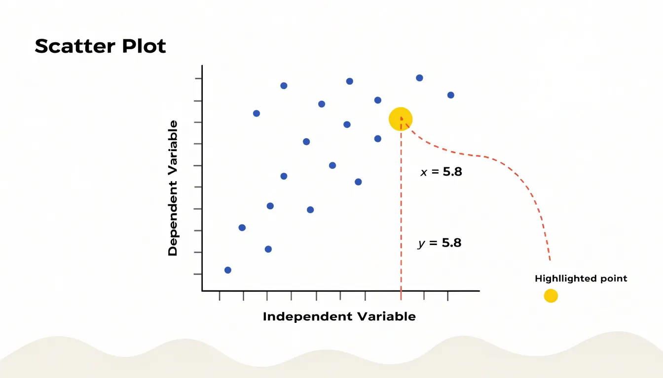
Each dot corresponds to one observation, positioned by its pair of values. To read a point, move straight down to the X-axis to find its horizontal value, then straight across to the Y-axis for its vertical value. Plotting many paired points turns a table into a visual pattern, revealing how the two variables move together.
The axes also establish scale and range. Tick marks divide each axis into intervals, affecting how spread out or compressed the point cloud appears. Consistent, clearly labeled axes with units make the plot interpretable and allow comparison across charts. Reading a scatter plot comes down to three habits: identifying the variable on each axis, locating individual points by their coordinates, and noticing the overall shape formed by all points together.
Preparing Data Pairs
Preparing data pairs begins with identifying the two columns that will become the X and Y axes, then verifying that each row represents a single observation with one value in each column. When data arrives from separate sources, such as a measurement table and a results table, rows often need to be joined on a shared identifier like a sample number or timestamp. Joining on the wrong key, or on a non-unique key, is a common way mismatched pairs slip into an analysis. Confirming uniqueness on the join key before merging protects against silent row duplication.
Cleaning comes next:
- Missing values: A row with an X-value but no Y-value cannot be plotted. Dropping only the missing cell rather than the whole row shifts every subsequent value out of alignment. Filter out entire rows where either variable is missing so remaining rows keep their original pairings intact.
- Formatting issues: Convert text placeholders such as
"N/A","null", or empty strings into true missing values before filtering. Standardize numbers stored as text, stray whitespace, and inconsistent decimal separators so values sort and plot correctly. - Duplicates and outliers: Decide deliberately whether a duplicated observation is a genuine repeated measurement or a data entry error, as this choice affects the visual weight it carries in the plot.
Once the table contains complete, aligned pairs, run a quick sanity check: confirm the row count, verify the minimum and maximum of each variable against expectations, and spot-check a handful of rows by hand.
Positive Trends
When points drift upward from left to right, the scatter plot shows a positive association: as values on the horizontal axis increase, values on the vertical axis tend to increase as well.
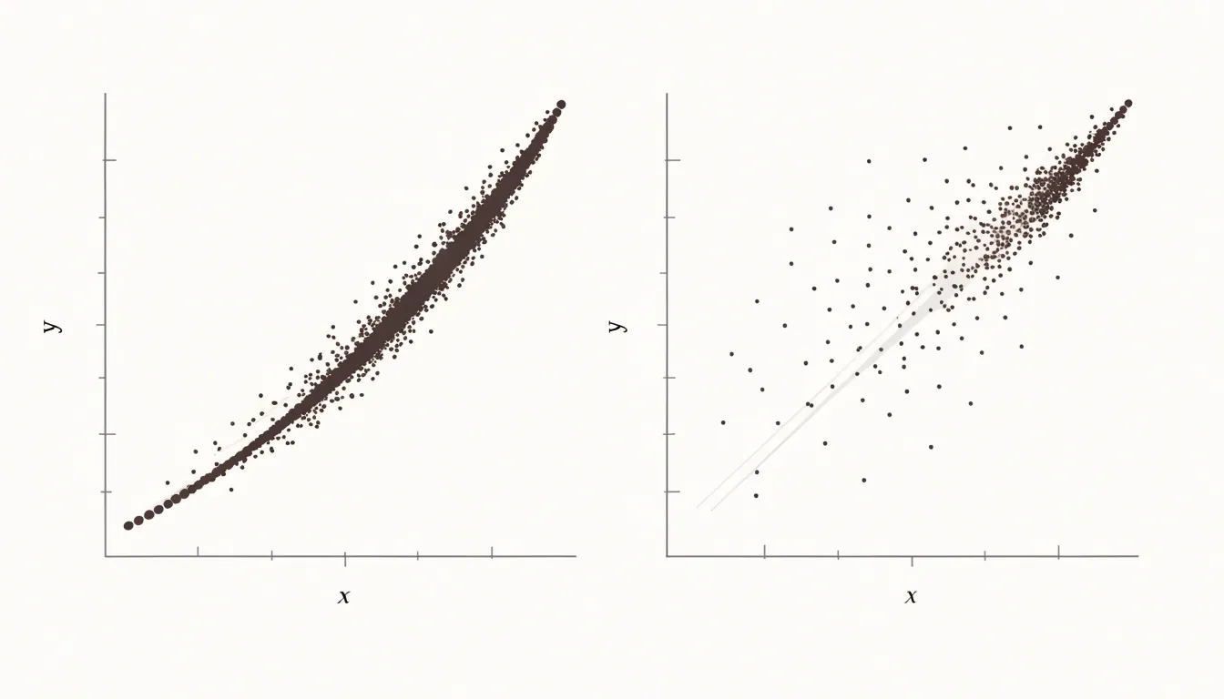
The points do not need to fall on a perfect line, and some scatter is expected, but a steady rise across the plot signals that the two variables move in the same direction. Several visual cues confirm this judgment:
- The densest cluster of points slopes upward.
- The vertical position of the point cloud at the left edge sits noticeably lower than at the right edge.
- An imaginary line drawn through the center of the points rises from left to right.
In fields from economics to biology, variables that rise together invite questions about cause and mechanism, showing where increases in one measure track increases in another.
Negative Trends
A negative trend appears when points slope downward from left to right: higher values on the horizontal axis pair with lower values on the vertical axis. As one quantity grows, the other shrinks.
Everyday examples illustrate this trade-off:
- Transportation: Plotting car speed (X-axis) against travel time for a fixed distance (Y-axis) shows points falling steadily as speed rises.
- Manufacturing: Higher machine operating temperatures often correspond to shorter component lifespans.
- Retail: Larger product discounts frequently line up with smaller profit margins per unit.
- Agriculture: Greater shade over a plot tends to accompany lower crop yields.
The steepness of the downward slope carries useful information. A steep negative trend signals that small changes in one variable accompany large changes in the other, while a gentle slope suggests a weaker linkage.
No Correlation
When data points form a diffuse, cloud-like cluster without clustering along a line, arc, or other recognizable shape, the variables vary independently of one another. A value on one axis tells you essentially nothing about the likely value on the other. A classic example is height versus intelligence test scores in a general population: tall people are not reliably smarter or less smart than short people, so the plotted points scatter broadly without directional drift.
Distinguishing genuine randomness from a weak or hidden pattern requires looking at sample size, since small samples can produce scattered clouds that mask real trends. Correctly spotting no correlation prevents analysts from wasting resources building predictive models on unrelated variables or drawing unwarranted causal conclusions.
Trendlines
A trendline is a straight line drawn through a scatter plot to capture the general direction of the data. It is typically calculated using least squares regression, which finds the line of best fit by minimizing the total squared distance between each point and the line. Most spreadsheet tools and charting libraries compute this automatically. The line takes the form $y = mx + b$, where $m$ is the slope describing how steeply the trend rises or falls, and $b$ is the intercept showing where the line crosses the vertical axis.
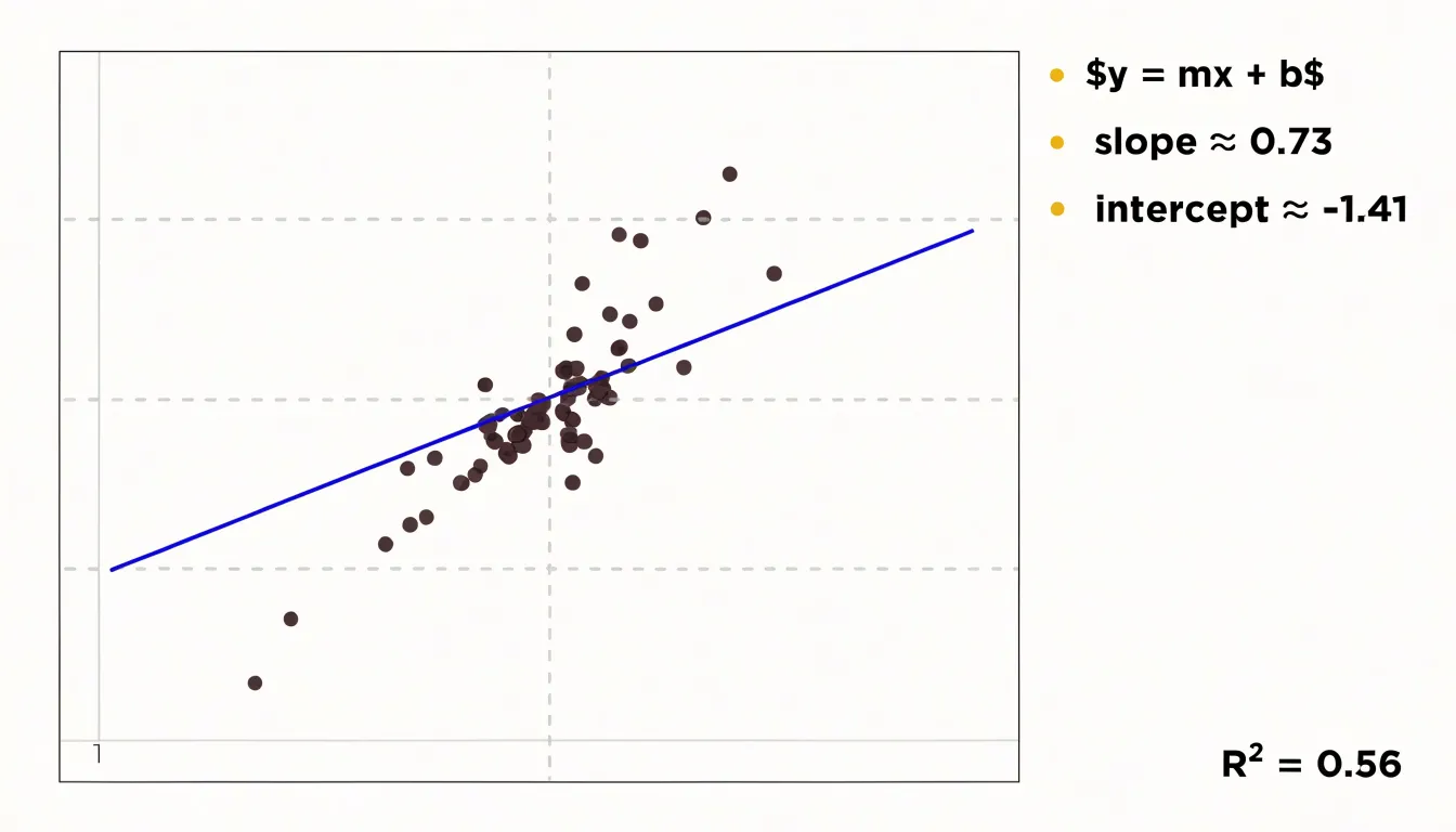
The trendline smooths out the noise of individual observations to provide an expected Y-value at any given X-value. By extending the line beyond the range of plotted points, you can extrapolate to estimate future or unmeasured values. This works best when the underlying relationship is genuinely linear and the data is tightly clustered around the line. Many tools also display the coefficient of determination ($R^2$), which quantifies how well the line fits the data, with values closer to 1 indicating a stronger fit.
Outliers
Outliers are points that sit isolated from the main cluster of the plot. They demand attention because a single extreme value can pull a trendline, inflate a correlation coefficient, or distort the visual pattern. Some outliers are obvious at a glance, lying far along an axis or in an empty region. Others reveal themselves only after fitting a line or computing residuals, since a point can have an unusual combination of X and Y values without being extreme on either axis alone.
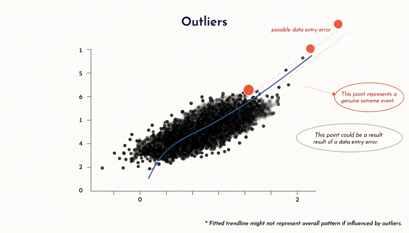
Once an outlier is identified, investigate its root cause by checking raw records, collection procedures, and domain plausibility. Common causes include:
- A data entry error, such as a misplaced decimal.
- A sensor failure recording an impossible reading.
- A genuinely rare event, like a market shock or record-breaking performance.
- A subgroup of the population behaving differently from the rest.
Remove the point only when the value is demonstrably erroneous and cannot be corrected, and document the removal to keep the analysis transparent and reproducible. When an outlier reflects a real phenomenon, retain it and consider reporting results both with and without the point to show how much influence it carries.
Relationship Strength
The strength of a relationship is read by observing how tightly points cluster around the trend running through them. A tight band of points following a clear path signals a strong, dependable association, while a wide, diffuse spread indicates a weak one.
This visual judgment connects directly to statistical correlation coefficients such as Pearson’s $r$:
- Near $+1$ or $-1$: Points cling closely to a rising or falling line (e.g., $r = 0.9$ looks like a narrow, cigar-shaped band).
- Near $0$: Points form a shapeless cloud, while $r = 0.3$ looks like a broad, fuzzy oval.
Analysts should read the plot and the coefficient together. A high $r$ can be artificially inflated by a few distant outliers, which the plot immediately reveals. Conversely, a coefficient near zero only measures linear correlation and can hide a strong non-linear relationship, such as a U-shaped curve. Separate subgroups within the data may also show strong internal trends while producing a weak combined coefficient.
Correlation vs. Causation
A tight cluster of points sloping upward or downward shows only co-variation—that two quantities move together across observed cases. It does not prove that one variable causes the other.
Confounding variables are the most common reason a clean pattern misleads. For example, a plot showing cities with higher ice cream sales also reporting higher drowning rates displays a convincing upward trend, yet warm summer weather raises both independently. Hidden factors like income, geography, or measurement practices can similarly drive two unrelated quantities into a shared trend.
Several logical traps compound the problem:
- Post hoc reasoning: Assuming that because one event followed another, the first caused the second.
- Fallacy of the single cause: Crediting one visible variable while ignoring a wider web of influences.
- Selection effects: Gathering a sample in a way that favors certain cases, creating an artificial cluster that reflects data collection rather than a true relationship.
Treat a strong visual association as a prompt to ask what else might explain the relationship, whether the direction of influence could run in reverse, and whether a controlled study can separate competing explanations.
Non-Linear Patterns
Real-world data frequently forms curved shapes that a straight line cannot describe:
- Exponential growth: Points rise slowly at first and accelerate upward, bending more steeply as X-values increase (common in population growth, compound interest, and early disease spread).
- U-shaped patterns: Values fall to a low point and climb again, typical of phenomena that perform best at moderate levels and worse at both extremes.
- Logarithmic curves: Points rise quickly at low values and then flatten out.
- S-shaped curves: Points transition smoothly between low and high plateaus.
Look for systematic bending or shifting rates of change across the data range. A residual plot can confirm the impression: a curved arrangement of residuals around the zero line signals that a linear model leaves structure unexplained.
To model a non-linear shape, fit a smooth curved function—such as a polynomial, exponential, or logarithmic curve—or transform an axis, such as plotting one variable on a logarithmic scale so exponential growth appears as a straight line.
Multiple Categories
Assigning color or marker shape to a third, categorical variable—such as region, product line, or experimental condition—lets multiple groups share one coordinate space. Readers can trace the aggregate trend while seeing how subgroups cluster, overlap, or diverge.
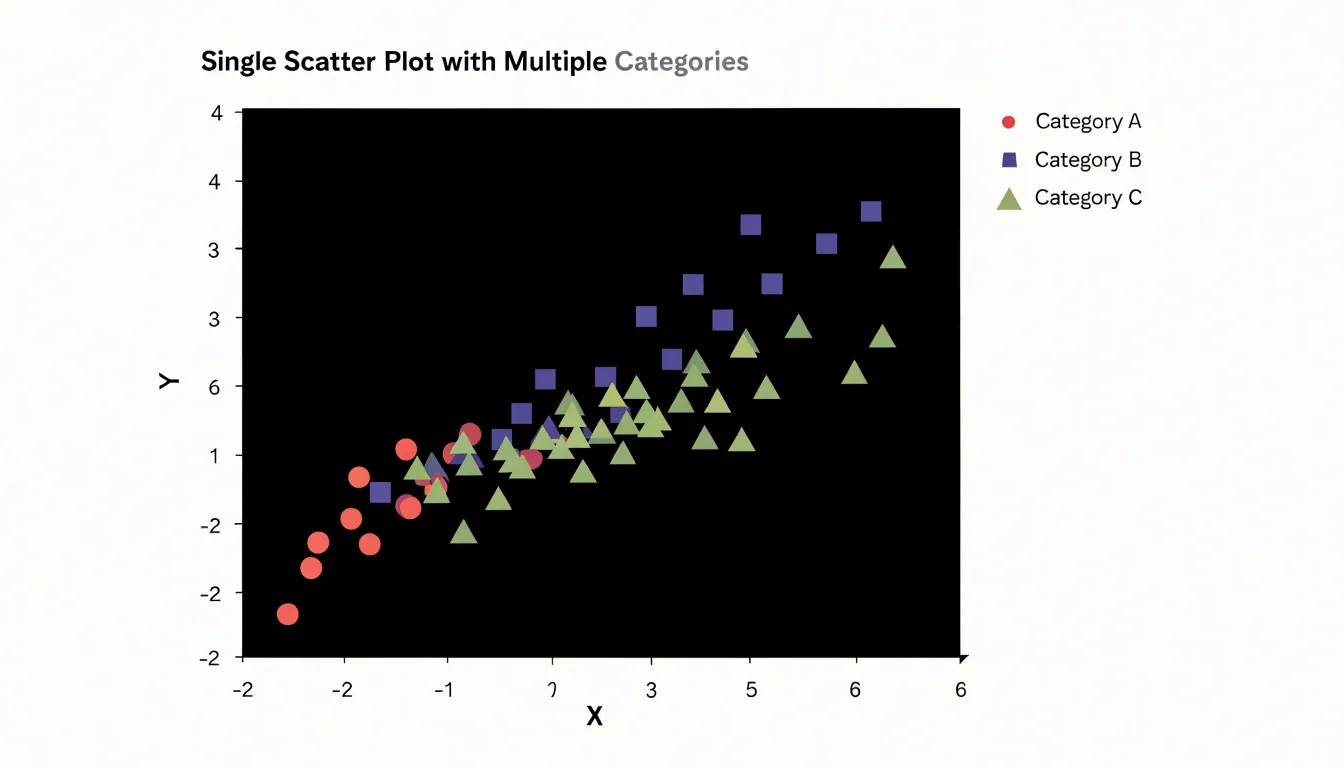
- Color: Works best for categories with a modest number of levels, since the human eye can reliably distinguish about five to eight hues. Use a restrained palette and reserve the most saturated color for the category of greatest interest.
- Shape: Marker forms such as circles, squares, triangles, and diamonds remain distinguishable in grayscale printing and for viewers with color vision deficiencies. Combining color with shape encodes two categorical variables at once (e.g., color for region, shape for time period).
Position the legend close to the plotted data and order it to match the analytical narrative. When categories multiply, keep markers small and use transparency to prevent overplotting.
Axis Scaling
Axis scaling determines how accurately a scatter plot represents the geometry of the data:
- Axis ranges: Each axis should span the full spread of data points with a small margin near the extremes. A narrow range clips observations at the edges, while an overly wide range compresses points into a small, unreadable cluster.
- Truncated axes: Starting a vertical axis well above zero can exaggerate small differences, making a modest association appear steep and dramatic. Compressing or stretching the horizontal axis similarly alters the apparent slope and visual density. Where a non-zero baseline is necessary, label it clearly so readers understand the frame of reference.
- Interval spacing: Place tick marks at regular numeric increments (such as steps of 1, 5, 10, or 50) so equal distances on the page correspond to equal differences in value. If a logarithmic transformation is used, explain it clearly on the axis.
Common Mistakes
- Overplotting: When many data points overlap, they obscure individual values and underlying patterns. Fix this by reducing marker size, increasing transparency (alpha) so dense regions appear darker, or switching to hexbin or 2D histograms for very large datasets.
- Cluttered labels: Too many text labels, tick marks, or gridlines make a plot unreadable. Label only key points, use interactive hover labels, rotate or abbreviate axis text when necessary, and remove unnecessary gridlines.
- Mislabeled axes: Omitting units, using cryptic abbreviations, or mismatching variable names causes confusion. Always include descriptive titles and units.
- Improper scale choices: Using a linear scale for data spanning orders of magnitude compresses small values; use a logarithmic scale instead.
Building Scatter Plots in Spreadsheets
To create and customize a scatter plot in Microsoft Excel or Google Sheets:
- Organize the data: Place the independent variable (X-axis) in the left column and the dependent variable (Y-axis) in the adjacent right column. Select the data range, including headers.
- Insert the chart: In Excel, go to the Insert tab, locate the Charts group, click the Scatter chart icon, and choose the basic scatter plot. In Google Sheets, click Insert > Chart and select Scatter chart from the Chart type dropdown.
- Format the layout: Double-click the chart to open the formatting pane. Add a descriptive chart title, label both axes, and adjust scales and gridlines. Change marker style, size, and color to highlight data points or add data labels for key observations.
- Add a trendline: In Excel, right-click any data point, select Add Trendline, choose a model (linear, exponential, logarithmic, etc.), and check the options to display the equation and $R^2$ value on the chart. In Google Sheets, find these options under the Customize tab in the chart editor.
Real-World Examples
Walking through concrete scenarios shows how direction, spread, and outliers work together in practice:
- Advertising spend vs. revenue: Plotting monthly ad spend (X-axis) against revenue (Y-axis) lets a marketing team check whether higher spend accompanies higher revenue and whether diminishing returns bend the trend into a curve. A month with unusually high revenue for modest spend stands out as an outlier, prompting investigation into whether a seasonal promotion, viral campaign, or data entry error occurred.
- Study hours vs. test scores: Plotting hours studied against exam results for a class typically reveals a positive trend, but the spread around the trend is instructive. Two students who both studied five hours may earn very different scores, illustrating that study time does not solely determine the outcome and raising questions about whether the pattern holds across different courses.
Frequently Asked Questions
How do I decide which variable goes on the X-axis and which goes on the Y-axis in a scatter plot?
The horizontal X-axis typically carries the independent variable—the quantity you control, observe, or use as a reference—while the vertical Y-axis usually carries the dependent variable. Deciding which variable belongs on which axis is the first step in constructing the plot.
How should I handle missing values when preparing data pairs for a scatter plot?
Filter out entire rows where either variable is missing so the remaining rows keep their original pairings intact. Dropping only the missing cell rather than the whole row shifts every subsequent value out of alignment.
What does a negative trend look like on a scatter plot?
A negative trend appears when points slope downward from left to right: higher values on the horizontal axis pair with lower values on the vertical axis. As one quantity grows, the other shrinks.
How is a trendline on a scatter plot calculated?
A trendline is typically calculated using least squares regression, which finds the line of best fit by minimizing the total squared distance between each point and the line. The line takes the form (y = mx + b), where (m) is the slope and (b) is the intercept.
What should I do if I find an outlier in my scatter plot?
Investigate its root cause by checking raw records, collection procedures, and domain plausibility. Remove the point only when the value is demonstrably erroneous and cannot be corrected, and document the removal; when an outlier reflects a real phenomenon, retain it and consider reporting results both with and without the point.
Can a scatter plot prove that one variable causes another?
A tight cluster of points sloping upward or downward shows only co-variation—that two quantities move together across observed cases—and does not prove that one variable causes the other. Treat a strong visual association as a prompt to ask what else might explain the relationship, whether the direction of influence could run in reverse, and whether a controlled study can separate competing explanations.
Tony Astor
Tony writes about data visualization and the tools people use to build charts and dashboards. More about Data Illustrator