Sankey vs Chord Diagram: Visualizing Flows and Links
 By Tony Astor ·

Sankey vs Chord Diagram
A Sankey diagram shows a directed flow through sequential stages, using proportional band widths to reveal quantities, losses, and splits along a linear path. A chord diagram arranges categories around a circle and connects them with interior ribbons, emphasizing many-to-many relationships and reciprocity. Choose Sankey for directional processes; choose chord for interconnected networks.
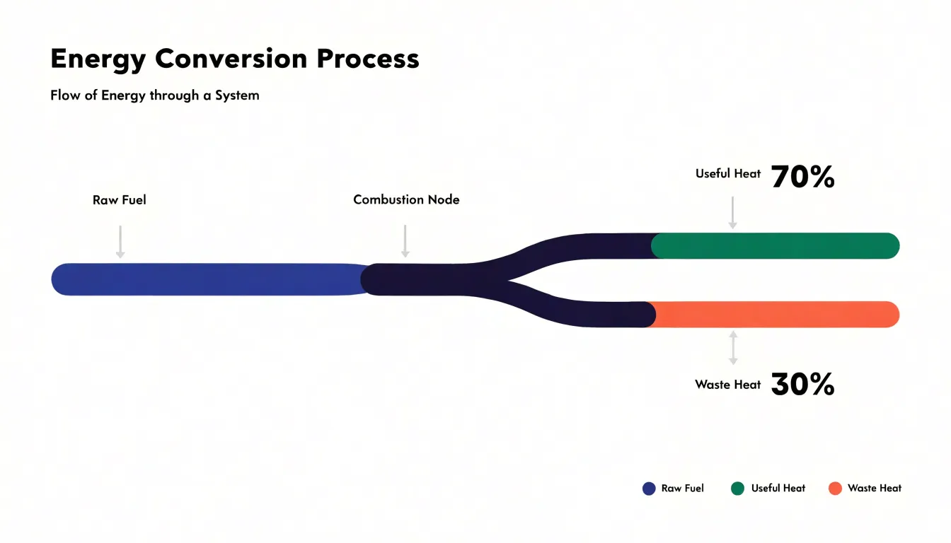
Table of Contents
Sankey Diagram
A Sankey diagram maps the sequential progression of a quantity from its source to its final destination through a series of discrete processing stages. Each stage is represented as a vertical node, and the connections between nodes are drawn as flowing bands whose thickness is directly proportional to the volume or energy passing through that transfer point. This visual encoding makes it immediately apparent how much of the original input survives each stage, where losses occur, and how the flow splits or merges along the way. For example, in an energy conversion system, the diagram might start with a thick band of raw fuel input, which then narrows as it passes through a combustion stage, splits into useful heat and waste heat, and further divides as the useful heat is distributed to different end uses. Because the width of each band is quantitative, viewers can compare the magnitude of flows at a glance, identifying dominant pathways and bottlenecks without needing to read numerical labels. The sequential layout reinforces the directional nature of the process, guiding the eye from left to right (or top to bottom) along the chain of transformations. This makes Sankey diagrams particularly effective for communicating efficiency, loss, and allocation across multi-step systems, where the cumulative effect of successive stages is central to the story. By preserving the continuity of flow from source to sink, the diagram highlights the interconnectedness of stages and the overall balance of the system, allowing stakeholders to trace how a particular input is distributed and where interventions might yield the greatest impact.
Chord Diagram
A chord diagram arranges its categories as segments distributed around the circumference of a circle, with each segment occupying a portion of the perimeter that typically reflects its total magnitude. The circular layout gives every category equal visual standing, since no segment is privileged with a top or starting position. Once the segments are placed, ribbon-shaped links are drawn across the interior, connecting pairs of segments whose values are related. Each ribbon spans from one segment to another, and its width at each endpoint is proportional to the flow or shared quantity between those two categories. Where the connection runs in both directions, the ribbon is usually split into two bands that meet in the middle, so the reader can see the volume traveling each way without the two flows obscuring one another.
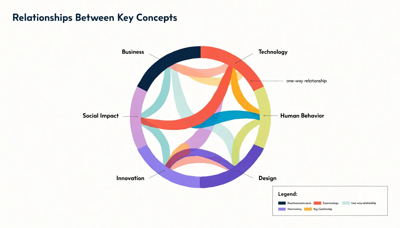
The circular arrangement is what gives the chord diagram its particular strength. Because links cross the open interior rather than stacking along an axis, the form naturally accommodates bilateral relationships, where two categories exchange volume, and multi-directional relationships, where a category connects to several others at once. A single segment can carry many ribbons, each of a different width, which makes it possible to read at a glance how a category’s total activity is divided among its partners. The result is a compact picture of mutual dependence: the perimeter shows how much each category holds, and the ribbons show how that volume is shared.
Reading a chord diagram involves tracing a ribbon from one segment to another and comparing its width with the widths of neighboring ribbons. The eye follows the arcs and chords as a connected system, picking out which pairs are tightly linked and which categories act as hubs with many connections. This makes the chart well suited to datasets such as trade between countries, migration between regions, or interactions within a network, where the question is fundamentally about who is connected to whom and how much passes between them.
Sankey Diagram
A Sankey diagram is built from three core structural elements: nodes, links, and widths. Nodes are typically drawn as rectangles and represent the entities or stages in the flow system—such as departments, processes, or categories. Each node acts as a collection point for flows entering and leaving, and its vertical extent is determined by the total flow volume passing through it. Links are the curved bands connecting nodes, and they represent the movement of a quantity from one node to another. The width of each link is proportional to the quantitative value it carries, so a link twice as wide as another indicates twice the flow volume. This proportional width is the primary visual encoding in a Sankey diagram, allowing viewers to compare magnitudes directly. The mechanics of a Sankey diagram rely on conservation of flow: the total width of incoming links at a node equals the total width of outgoing links, unless the node is a source or sink. This principle ensures that the diagram maintains a balanced and accurate representation of the underlying data. In practice, node heights are often set to accommodate the total flow, and link widths are scaled accordingly. The layout algorithm arranges nodes along a horizontal axis, typically from left to right, minimizing link crossings and maintaining clarity. The combination of rectangular nodes, proportional links, and flow conservation creates a powerful visual tool for understanding complex systems, where the thickness of each connection immediately communicates the relative importance of different pathways.
Chord Diagram
A chord diagram arranges its categories as segments along a single circular axis. Each segment occupies a portion of the outer ring, and the angular width of that portion is proportional to the total value associated with the category it represents. This outer ring therefore works as a compact summary of totals: a reader can compare the relative size of every category at a glance by comparing arc lengths around the perimeter. The ring also provides anchor points, since every relationship in the dataset begins and ends somewhere on this same circle.
Inside the ring, ribbons connect one arc segment to another. A ribbon’s width at each end is scaled to the volume of flow between the two categories it links, so the ribbon tapers or widens along its path when the two directional values differ. The curvature of the ribbon carries the eye from source to destination, and the layering of many ribbons over one another produces the dense interior weave that gives chord diagrams their characteristic appearance.
Self-flows, where a category exchanges value with itself, appear as small loops that emerge from a segment and curl back into the same segment. These loops sit close to the outer ring and keep internal circulation visible rather than hiding it. Asymmetrical connections are handled by letting the two ends of a ribbon take different widths, which preserves the direction and magnitude of each side of the exchange. Color is typically assigned per category and applied to both the segment and the ribbons leaving it, so a reader can trace a flow from its origin around the circle and across the interior to its destination, following both total size and pairwise volume in one integrated view.
Sankey vs Chord
Sankey diagrams and chord diagrams approach the visualization of complex relationships through fundamentally different spatial architectures. A Sankey diagram arranges its data along a horizontal axis, with flows progressing from left to right in a linear sequence. Nodes sit at fixed positions along this axis, and the banded links between them carry a visual weight proportional to their value. This linear structure mirrors a narrative of movement, where a viewer reads the diagram much like a page of text, following each stream from its origin toward its destination. The geometry reinforces directionality, and the consistent horizontal rhythm makes it easy to trace a single pathway across multiple stages without losing one’s place.
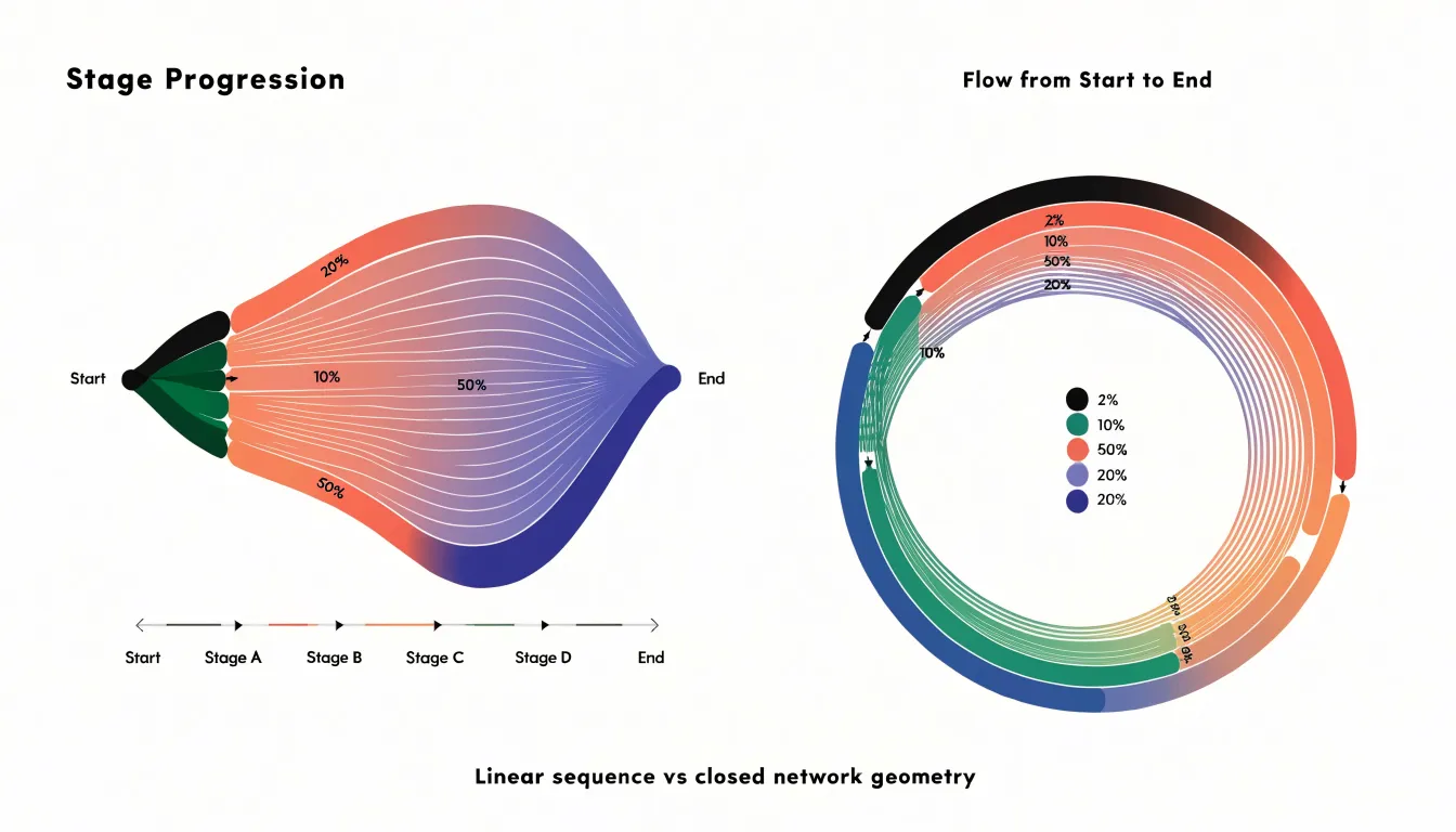
A chord diagram instead arranges its nodes around the perimeter of a circle and draws connections across the interior. This radial layout treats every node as part of a closed network, where relationships run in both directions and no single flow claims primacy over another. The circular arrangement emphasizes the interconnectedness of the whole system, and the interior chords create a dense web that reveals patterns of reciprocity and mutual exchange.
These contrasting geometries carry practical consequences for readability and spatial efficiency. The linear layout of a Sankey diagram excels when the data has a clear directional logic, such as energy transfer, budget allocation, or supply chains, because the eye can follow a stream across successive stages with minimal effort. Its horizontal extent grows with the number of stages, which can demand significant screen width for deep hierarchies. The circular layout of a chord diagram compresses many pairwise relationships into a compact footprint, making efficient use of space when the dataset involves dense many-to-many connections. However, the crossing chords inside the circle can produce visual clutter as density increases, and tracing a single connection across the interior requires more careful attention than following a straight horizontal band. The choice between the two therefore rests on whether the underlying structure is a directed sequence or a closed network.
Sankey Diagram
A Sankey diagram excels when information moves in a single direction through a sequence of connected stages. The classic use case is a process with a defined beginning, a series of intermediate steps, and a clear endpoint. Picture a customer journey that starts with a website visit, passes through product views, cart additions, checkout initiation, and purchase completion. Each of these stages can be represented as a node, with the width of the connecting bands proportional to the volume of users or units flowing through. This makes it immediately obvious where the largest volumes travel and where the stream narrows.
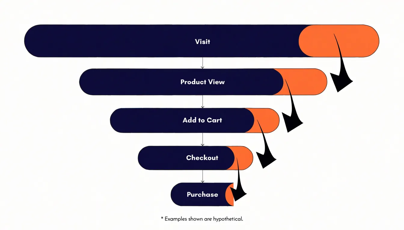
That narrowing is where Sankey diagrams earn their keep. Because every band’s thickness maps directly to a quantity, tracking drop-offs becomes a visual exercise rather than a numerical one. A sudden contraction between two nodes signals a stage where many users abandon the process, and the relative size of that contraction tells you how severe the loss is compared with other stages. Conversion rates emerge from the same logic, since the ratio between the width entering a stage and the width leaving it can be read at a glance across the whole pipeline.
Sequential distribution is another area where this chart type shines. When a total population splits into sub-groups at each stage, the branching bands show how those sub-groups shrink, merge, or persist as they progress. Budget allocations moving through departmental approvals, energy losses across a conversion chain, or candidate attrition through a hiring funnel all fit this pattern. The key requirement is directional flow with ordered stages, so the reader can follow a path from origin to outcome without ambiguity.
Chord Diagram
Chord diagrams excel at revealing the texture of relationships among a fixed set of entities, where every participant can in principle exchange value with every other. This makes them a natural fit for matrix-style data: origin-destination tables, migration flows between regions, trade between countries, or communication traffic between departments. Once the data is arranged as a square matrix, the diagram renders each entity as an arc around a circle, with ribbons connecting pairs. The width of each ribbon encodes the volume of the exchange, and the arcs terminate in proportions that show how much each entity sends or receives overall. Readers can therefore scan the full picture and see, at a glance, which connections carry the most weight.
One of the diagram’s strongest qualities is its ability to expose dominant clusters. When several entities exchange heavily among themselves, their ribbons bunch into a dense visual cluster that immediately signals a subgroup of tightly coupled participants. Reciprocal exchanges also stand out clearly: two ribbons running between the same pair of arcs make the mutual nature of the relationship visible in a way that a one-directional chart cannot convey. This matters in analyses of partnership, referrals, or two-way trade, where the balance between what flows out and what flows back is central to the question.
Chord diagrams also handle cross-group overlaps gracefully. Because every entity shares the same circular frame, ribbons that bridge distinct subgroups remain visible and measurable, showing where boundaries blur and where different clusters interlock. Analysts can trace which entities act as connectors, carrying volume between otherwise separate communities.
Use a chord diagram when the entity set is stable, the relationships are genuinely many-to-many, and the reader’s task is exploratory: finding the hubs, the tight knots, and the bridges in a network of exchanges. In those settings it turns a dense matrix of numbers into an immediate visual impression of structure.
Sankey Diagram
Sankey diagrams excel at visualizing flow and quantity through a system, making them invaluable for mapping supply chains. In manufacturing, a Sankey diagram can trace raw materials from procurement through each production stage, showing how inputs transform into intermediate goods and final products. For instance, a steel manufacturer might use one to track iron ore from the mine to the blast furnace, then to casting, rolling, and finished coils, with widths proportional to material volume. This reveals inefficiencies, such as excessive scrap at a particular stage, and helps optimize resource allocation.
In financial contexts, Sankey diagrams clarify budget allocations and cash flow. A government or corporation can depict revenue sources flowing into various expenditure categories, with branch widths representing amounts. This makes it easy to see how much of a budget goes to operations, marketing, or R&D, and how funding shifts over time. Investors might use Sankey diagrams to visualize portfolio flows, showing capital moving between asset classes or sectors.
For user journeys, Sankey diagrams map website or app navigation, highlighting conversion paths. Each node represents a page or action, and flows show the number of users moving between them. Marketers can identify drop-off points, such as a high exit rate on a checkout page, and optimize the funnel. By comparing flows before and after changes, teams can measure the impact of UX improvements.
Across industries, Sankey diagrams provide a clear, quantitative view of complex flows, enabling better decision-making and communication.
Chord Diagram
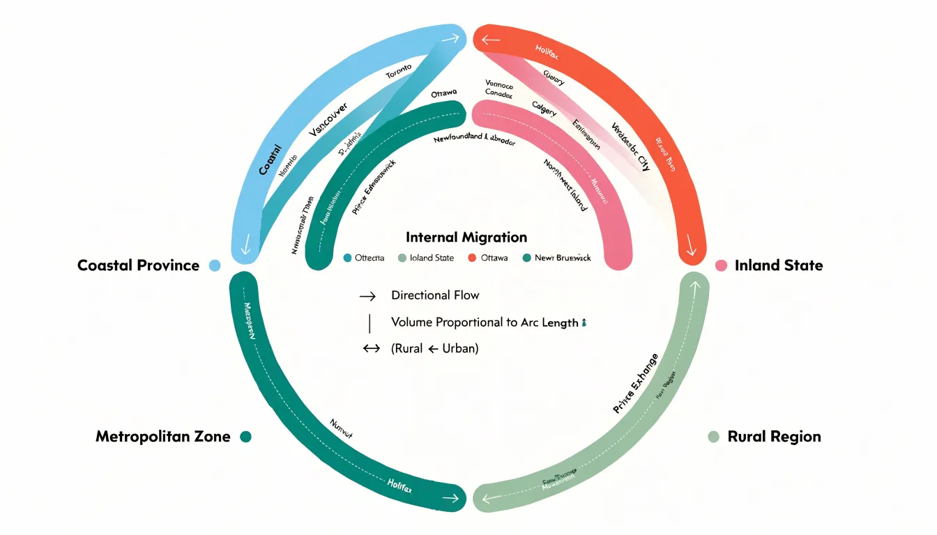
Chord diagrams excel at showing how entities flow between one another, and migration is one of the clearest practical examples. Picture a chart where each region of a country occupies a segment around the circle—a coastal province, an inland state, a metropolitan zone. Ribbons connecting these segments represent people relocating from one place to another over a census period. A thick ribbon from a rural region to an urban one immediately communicates a population drain, while reciprocal ribbons in both directions reveal balanced exchange. Planners and demographers can spot which regions act as net sources and which as net receivers, and the relative thickness of each arc shows the magnitude of movement without requiring readers to parse a dense table of numbers.
Global import-export dynamics offer another natural fit. Assign each country an arc, sized by total trade volume, then draw ribbons for bilateral flows of goods. A reader can trace, for instance, how manufactured goods travel from East Asia to North America and Europe, or how agricultural commodities move in the opposite direction. Because the ribbons preserve direction through the order of their endpoints, the diagram distinguishes exporters from importers at a glance. Economists use these visuals to illustrate trade dependencies, identify concentrated relationships between a handful of partners, and reveal imbalances where one side ships far more than it receives.
Social networks and online communities round out the use cases. Consider several distinct forums or platforms, each given an arc, with ribbons representing users who participate in more than one community. A heavy band between two forums signals substantial audience overlap, which matters for advertisers, community managers, and researchers tracking how discourse spreads. Interaction metrics such as shared membership, cross-posted content, or message exchanges can be plotted the same way. The chord layout makes clusters of closely tied communities visible, and isolated arcs highlight groups whose audiences rarely venture elsewhere.
Design Pitfalls
Design pitfalls in flow diagrams often begin with link crossing overload. When many connections intersect in a small area, the viewer’s eye loses its path and the diagram becomes a puzzle rather than an explanation. This typically happens when node placement follows data order rather than visual logic. A practical remedy is to reorder nodes so that heavily connected items sit near each other, grouping related categories along the axis and placing high-traffic nodes toward the center. Iterative node ordering, even by hand, can dramatically reduce crossings before any styling is applied.
Color is the second common failure point. Low contrast between adjacent links makes individual flows indistinguishable, while too many saturated hues create visual noise that competes with the data itself. Functional color schemes help here: use a restrained palette, reserve strong colors for the most important flows, and let secondary connections fade into muted tones. Consistent hue families for related categories reinforce grouping without adding clutter, and sufficient lightness contrast keeps thin links legible against the background.
Scale proportions introduce a subtler risk. When link widths or node sizes are drawn without matching the underlying quantities, viewers read false magnitudes. Proportional widths should be computed directly from the data, with a shared baseline so that comparisons across the diagram remain honest. Truncated scales or exaggerated minimum widths can make minor flows look significant and major ones look smaller than they are.
Together, these strategies form a checklist: order nodes to minimize crossings, choose colors that separate rather than decorate, and size every element from real values. Applied early, they keep the diagram readable and trustworthy.
Interactivity
Dense flow charts carry a great deal of information in a single view, and that density is precisely what makes them valuable and what makes them difficult to read. Interactivity resolves this tension by letting the chart hold a full dataset while revealing only the relevant slice at any given moment. Tooltips form the first layer of this strategy. When a reader hovers over a flow path, a node, or a junction, a small panel can surface the exact source, target, and magnitude behind that mark, along with derived values such as percentages of the total. This keeps the visual surface clean because labels do not need to be printed permanently on every ribbon or segment; the detail appears on demand, attached to the reader’s point of interest.
Highlighting adds a second layer. Hover states typically dim unrelated marks and bring the hovered element to full emphasis, so the eye is guided without any change to the underlying layout. Node filtering extends the same principle to entire categories: a reader can isolate one industry, region, or stage of a process and watch the chart redraw around the surviving connections. The reduction in visual noise is immediate, and the relationships that remain become far easier to trace.
Path-tracing ties these behaviors together into a comprehension tool. Following a single connection across several hops in a static diagram often means losing one’s place among overlapping ribbons. With interaction, selecting a node or path can illuminate the full chain from origin to destination while muting everything else, so the reader perceives the connection as a continuous thread rather than a scattered set of segments. Hover states, filters, and dynamic tooltips thus work as complementary instruments, each removing a different kind of clutter and each supporting the reader in building an accurate mental model of the flow.
Performance and Scalability
Handling hundreds of data connections in a browser chart places real demands on rendering pipelines, and the techniques chosen early in a project determine whether the visualization stays responsive as data grows. The first line of defense is aggregation. Grouping fine-grained connections into meaningful buckets, such as rolling minor flows into an “other” category or merging links that share a common source and target, reduces the number of graphical elements the browser must draw and maintain. Aggregation also improves readability, since dense thickets of overlapping links become harder to interpret well before performance degrades.
Threshold filtering works alongside aggregation by removing connections that fall below a chosen value or percentage. A common approach sets a minimum flow size so that only the most significant links are rendered, with the remainder summarized or omitted. Interactive filters let users adjust these thresholds on the fly, keeping the initial view light while preserving access to detail on demand. Filtering should be paired with clear labeling so viewers understand what has been excluded from the display.
The rendering technology itself carries substantial weight. SVG creates a distinct DOM node for every path and label, which makes styling and event handling straightforward but introduces overhead once element counts climb into the hundreds or thousands. Canvas draws to a single bitmap surface, avoiding per-element DOM costs and generally sustaining smoother frame rates with large link counts, at the price of more manual work for hit testing and interaction. Many teams adopt a hybrid: Canvas for the dense link layer, SVG for labels and controls that benefit from native accessibility and event handling. Whichever path is taken, lazy loading, throttled redraws on resize, and precomputed layout data all help keep load times and interaction latency within acceptable bounds.
Mobile Responsiveness
Mobile responsiveness determines whether a complex data visualization remains usable once it leaves the desktop. Sankey and chord diagrams are inherently wide: Sankey layouts spread flows across multiple columns, and chord diagrams arrange nodes around a full circle, both of which demand generous horizontal space. On a compact smartphone viewport, squeezing either layout to fit the screen produces unreadable labels, hairline links, and nodes too small to tap. Best practice begins with a scrollable container. Wrapping the visualization in a horizontally scrollable element preserves the full geometry at a comfortable scale, letting viewers pan across the diagram instead of shrinking it into illegibility. Fixed minimum widths on the inner chart and clear visual affordances, such as edge shadows or partial peeking of off-screen content, signal that more content lies beyond the viewport.
A second strategy involves collapsible nodes. Complex diagrams often carry dozens of nodes and hundreds of links; collapsing secondary nodes into summary aggregates reduces visual density while keeping the core relationships intact. Mobile users can expand individual nodes on demand with a tap, revealing detail only when they need it. This progressive disclosure keeps the initial view clean and lowers rendering cost on devices with limited processing power.
Where interaction remains impractical, simplified fallback chart types offer a reliable path. A stacked bar chart, a ranked list of flows, or a small-multiple series can convey the essential relationships of the original diagram in a format that reads naturally on a narrow screen. The fallback should be selected through responsive breakpoints or capability detection so that desktop users still receive the full Sankey or chord view. Combining these approaches, scrollable containers for geometry, collapsible nodes for density, and simplified fallbacks for constrained contexts, gives mobile audiences a coherent experience of data that was designed for much larger canvases.
Decision Checklist
A decision checklist helps you choose between a Sankey and a chord diagram by systematically evaluating your dataset, audience, and narrative goals. Start with dataset structure: Sankey diagrams require acyclic, hierarchical data where flows move in one direction, such as energy transfer or supply chains. Chord diagrams handle cyclic or undirected relationships, like trade between countries or social network connections. Next, consider your target audience. For audiences unfamiliar with network diagrams, Sankey’s linear flow is more intuitive; chord diagrams suit audiences comfortable with matrix-like representations. Define your primary narrative: Sankey emphasizes the magnitude of flows and their distribution across stages, while chord diagrams highlight interconnectivity and reciprocity. A step-by-step decision matrix can guide you: first, classify your data as directional or undirected. If directional, check for cycles; if none, Sankey is appropriate. If undirected or cyclic, chord is likely better. Then, assess audience familiarity: choose Sankey for general audiences when flows are the focus; choose chord for technical audiences when relationships are key. Finally, align with your narrative: for process tracking or budget allocation, Sankey; for partnership networks or trade balances, chord. This checklist ensures a deliberate choice that maximizes clarity and impact.
Frequently Asked Questions
What is a Sankey diagram used for?
A Sankey diagram maps the sequential progression of a quantity from its source to its final destination through discrete processing stages, with band thickness proportional to volume or energy. It is effective for communicating efficiency, loss, and allocation across multi-step systems and for directional flows with ordered stages.
What is a chord diagram best for showing?
Chord diagrams excel at revealing relationships among a fixed set of entities where every participant can in principle exchange value with every other, such as origin-destination, migration, trade, or communication data. They can expose dominant clusters, reciprocal exchanges, and cross-group overlaps.
What is the difference between a Sankey diagram and a chord diagram?
A Sankey diagram arranges data along a horizontal axis with flows progressing left to right in a linear sequence, while a chord diagram arranges nodes around a circle and draws connections across the interior. The choice between them rests on whether the underlying structure is a directed sequence or a closed network.
How do I reduce clutter in Sankey and chord diagrams?
Reorder nodes so heavily connected items sit near each other, use a restrained color palette with strong colors reserved for important flows, and compute proportional widths directly from the data. These strategies help address link crossing overload, low contrast, and false magnitudes.
How does interactivity help with dense Sankey or chord diagrams?
Interactivity helps dense flow charts by using tooltips to surface exact source, target, and magnitude on demand, highlighting to dim unrelated marks, and filters or path-tracing to isolate a category or full chain. This keeps the chart clean while preserving access to detail.
How can I make Sankey and chord diagrams usable on mobile and with large datasets?
On mobile, wrap the visualization in a horizontally scrollable container, use collapsible nodes for progressive disclosure, and provide simplified fallback chart types where interaction remains impractical. For large datasets, use aggregation, threshold filtering, and rendering choices such as Canvas for dense link layers and SVG for labels and controls.
Tony Astor
Tony writes about data visualization and the tools people use to build charts and dashboards. More about Data Illustrator