Sankey Diagram vs Alluvial Diagram: Differences Explained
 By Tony Astor ·

Sankey Diagram vs Alluvial Diagram
Sankey diagrams show conserved flows—energy, money, or mass—where inflows equal outflows at every node, with band width proportional to quantity. Alluvial diagrams track how categories or groups split, merge, and persist across time steps, emphasizing trajectories rather than conservation. Choose Sankey for aggregate conserved flows through a network; choose alluvial when strata must stay traceable across ordered stages.
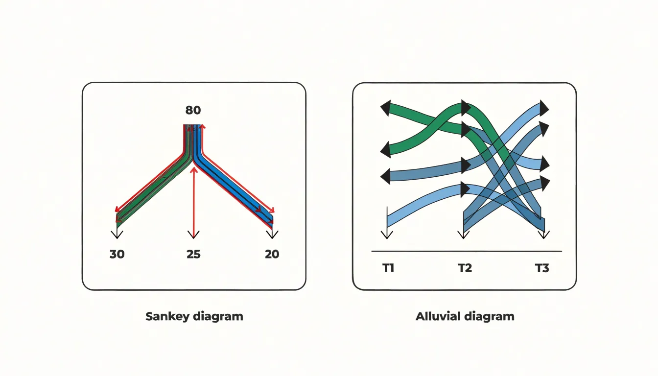
Table of Contents
Sankey Diagram
Sankey diagrams represent conservative transfer systems, where the total quantity of a resource remains constant as it moves between stages. The width of each flow is proportional to the magnitude of the quantity transferred, and the sum of inflows at any node equals the sum of outflows. This property of conservation makes Sankey diagrams effective for tracking energy and resource flows through complex processes, because the visual representation mirrors the underlying physical or accounting logic. When drawn correctly, a viewer can verify that no energy or material has been lost or fabricated at any stage, since the bands entering and leaving each node balance precisely.
In thermodynamic applications, Sankey diagrams map energy transformations in power plants, engines, and building systems. Inputs such as fuel or solar radiation are shown entering the system, while outputs include useful work, waste heat, and losses to the environment. Because energy is conserved, the diagram provides an immediate visual audit of where energy is consumed and where inefficiencies arise, helping engineers identify the largest loss pathways and prioritize improvements.
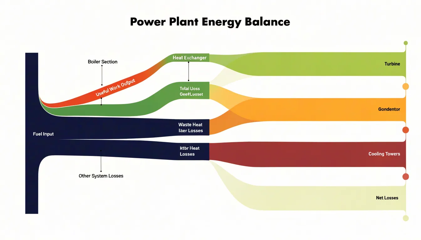
Industrial material flow analysis relies on the same principle. A Sankey diagram can trace raw materials through extraction, processing, manufacturing, use, and disposal, with each band representing a measurable mass. Since mass is conserved within the defined system boundary, discrepancies between inflows and outflows indicate measurement errors or unaccounted stocks, making the diagram a practical auditing tool.
Financial auditing offers another domain where conservative transfer logic applies. Currency moving through budgets, departments, or supply chains can be visualized as flows that must balance at each node, revealing where funds are allocated, redirected, or retained. The strict accounting identity underlying Sankey diagrams thus supports transparency and verification across thermodynamic, industrial, and financial contexts.
Alluvial Diagram
In an alluvial diagram, each stream traces the path of a group or cluster as it persists, splits, merges, or dissolves across a sequence of time steps or processing stages. The horizontal axis represents progression—months, years, project phases, or any ordered set of intervals—while the vertical axis distributes the members of each grouping at every step. The width of a stream is proportional to the number of entities it carries, communicating the relative size of that group at that moment. As the eye moves left to right, the changing widths and converging or diverging paths reveal how the composition of the underlying network or categorical set evolves.
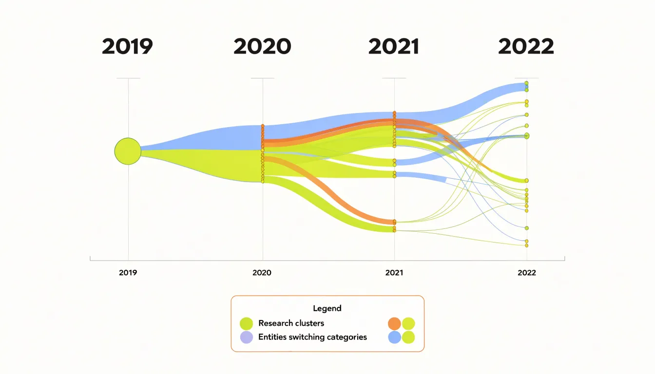
This structure answers questions about dynamics that static charts cannot easily address. A cluster that appears large at one stage may fragment into several smaller streams at the next, indicating a community breakup or a redistribution of categories. Conversely, separate streams may join into a single thick band, signaling consolidation or convergence. Entities that switch from one group to another are visible as streams that cross or bend toward a neighboring category, making reassignment and migration legible. This suits fields such as bibliometrics, where research clusters form and dissolve over publication years, or organizational analysis, where departments are restructured across reporting periods.
The ordering of nodes within each vertical column also carries meaning, since adjacent streams are easier to compare than distant ones. Designers typically arrange columns to minimize crossings and preserve continuity, so a reader can follow a single trajectory through the entire sequence. Labels at each column identify the clusters at that stage, accommodating renamed or newly created groups. By combining proportional flows with a temporal axis, the alluvial diagram turns structural change into a readable visual narrative of regrouping over time.
Flow Widths
Flow widths are the primary visual encoding in both Sankey and alluvial diagrams. The thickness of each link represents a scalar quantity, such as energy in megawatts, money in dollars, or people in thousands. Node heights are typically scaled to match the sum of incoming or outgoing flows, making the entire diagram a proportional map of magnitudes.
When widths are strictly proportional, a link twice as thick as another represents twice the quantity, allowing viewers to make precise comparisons without reading numbers. A glance reveals which pathways dominate and which are marginal. In complex systems with many nodes and crossing links, proportional widths maintain readability by giving visual weight to the most significant flows, letting viewers trace a path from source to sink and accumulate a sense of volume at each stage.
However, effectiveness depends on consistent scaling across the entire diagram. If widths are scaled independently for different parts, comparisons become misleading. Designers must also manage the trade-off between thickness and label space; very thin flows may become invisible, while very thick flows can dominate the layout. Interactive features like hover tooltips can supplement widths with exact values.
Time and Direction
Time and direction help determine which diagram type will serve a dataset best. When the underlying data describes a fixed sequence of stages, such as a customer moving from awareness to consideration to purchase, the structure is inherently static. Each stage represents a discrete checkpoint, and the focus rests on how volumes split and recombine across them. A Sankey diagram handles this scenario cleanly because its nodes and links can be laid out in a stable left-to-right order that mirrors the stage sequence without implying continuous motion. The reader sees proportions at each stage and understands the split as a snapshot rather than a journey in progress.
When the data instead captures continuous movement through time, the diagram must convey trajectories rather than simple stage transitions. Alluvial diagrams are built for this situation. Their links can be stretched along a horizontal axis to represent duration, and their crossings show how groups migrate between categories over successive periods. The visual emphasis shifts from static proportions to the path each entity follows, making the direction of movement explicit.
Consider a migration study tracking households across five census years. The data has genuine temporal continuity, and an alluvial layout lets viewers follow individual streams across years while seeing where they converge or diverge. A Sankey layout would flatten that continuity into stage buckets and lose the sense of progression. Conversely, a supply chain with fixed processing steps gains clarity from the Sankey approach, since the steps are ordered but not time-based in a continuous sense. The deciding question is whether the dataset describes stages that can be treated as discrete snapshots or movement that unfolds along a timeline.
Node Structure
Node structure in Sankey and alluvial diagrams shapes how information flows across the page. In a standard layout, nodes typically function as grouped columns, where each vertical arrangement represents a discrete categorical block. These blocks collect multiple flows into a shared band, so a single column might hold several related categories stacked one above the other.
This grouping creates a clear visual hierarchy, allowing a reader to scan down a column and compare the relative volume of each category within that block. The width of each node segment corresponds to the total flow passing through it, and the stacked arrangement makes aggregate quantities easy to assess at a glance. The column serves as a container that anchors several related streams, and the links between columns show how volume redistributes from one category set to the next.
A node structured as a single source point acts quite differently. Here the node represents one distribution hub—a singular origin from which many branches emerge. Rather than collecting several categories into a stacked band, the point-source node concentrates all outgoing flow at one location, and the diagram radiates outward from that center. This layout emphasizes the origin itself as the dominant element, with the width of the node reflecting total volume leaving that hub. Readers trace individual branches away from the point to see where the flow disperses. The visual weight sits at the source, communicating a spreading or fanning pattern rather than a side-by-side comparison of grouped items. Choosing between grouped columns and single point-source hubs depends on whether the diagram needs to compare categories within a block or highlight dispersal from one concentrated origin.
Splits and Merges
The defining behavior of a flow diagram is what happens to a path as it crosses from one categorical dimension to the next. In a Sankey diagram, each node acts as a junction where an inbound quantity is partitioned among several outbound links. Because inflows and outflows balance, a stream of 100 units may divide into 60 and 40, and each sub-flow carries its provenance forward as a discrete band. Visually this appears as a widening fan or a narrowing funnel at the node boundary, with the ribbon thickness at any point encoding the quantity still traveling together.
Merging is the mirror operation. When several sources feed a single destination, their ribbons converge into one node and exit as a consolidated stream. Because thickness is preserved through the junction, the viewer can read both the combined total and the individual contributions, provided the incoming bands retain their separate colors or ordering. The visual logic depends on consistent vertical stacking: sub-flows are usually ordered by their position at the previous node so a reader can trace a single band across multiple hops without losing it in the bundle.
Alluvial diagrams extend this logic to longitudinal data, where the same entities are measured across successive time points. Here splits and merges accumulate over many dimensions, and a single category may fragment into dozens of descendants or absorb many predecessors. The branching structure itself becomes the analytical object, revealing which groups persist intact, which dissolve, and which coalesce. Good design preserves band identity through every junction, since the graphic’s credibility rests on a reader’s ability to follow one thread from origin to terminus through all its divergences and consolidations.
Use Cases
Sankey diagrams excel in engineering and energy contexts where mass and energy balances must be tracked with precision. In a chemical plant, a Sankey diagram can map the flow of raw materials through reactors, separators, and recycle loops, quantifying losses at each stage. Similarly, energy analysts use them to visualize primary energy sources, conversion efficiencies, and final consumption across sectors, highlighting where energy is lost as heat. These applications demand strict conservation of flow, serving as a quantitative tool for optimization and auditing.
In contrast, alluvial diagrams are well-suited to categorical data science, particularly in analyzing user cohorts and machine learning classification paths. An alluvial diagram can trace how different user segments (e.g., new vs. returning users) transition between engagement states over time, such as from browsing to cart to purchase, with each category represented as a node and flows showing transitions. In machine learning, alluvial diagrams can illustrate the paths of instances through a decision tree or the evolution of predicted classes across model iterations, where the focus is on the proportion of items moving between categories rather than conserving a physical quantity. The flexibility of alluvial diagrams allows for multiple categorical dimensions and non-conservative flows, making them ideal for exploring complex categorical relationships and cohort dynamics.
Change Over Time
Because alluvial diagrams represent how a population moves through a series of stages, they are a natural fit for customer journey analysis. Each vertical bar represents a snapshot of the customer base at a given point in the sequence—whether a billing cycle, a product tier, or a discrete platform interaction. The connecting ribbons show how individuals or cohorts transition from one state to the next. When a ribbon narrows dramatically between two stages, the viewer immediately sees where attrition is concentrated. Churn becomes a visible outflow rather than an abstract percentage, and stakeholders can trace which segments or entry points feed most heavily into that outflow.
Upgrade paths benefit from the same structure. A customer who moves from a free tier to a paid plan and later to an enterprise subscription produces a continuous ribbon that winds through each stage, and the relative thickness of parallel paths reveals which upgrade routes carry the most traffic. Analysts can compare cohorts that entered at different times and observe whether the shape of the flow changes as the product matures.
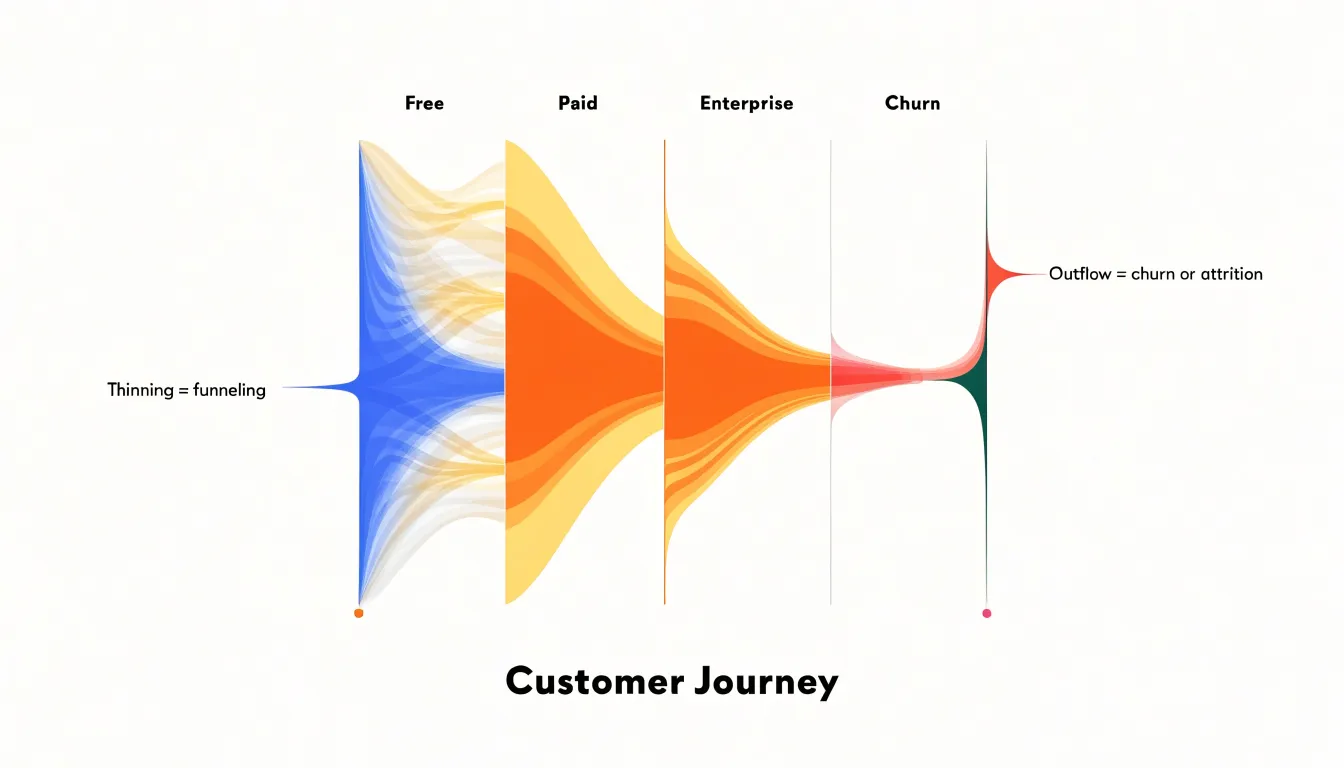
Multi-touch attribution funnels extend this logic to marketing and engagement sequences. By treating each touchpoint as a stage, alluvial flows show how prospects distribute themselves across channels before converting, and where they drop out along the way. Because the ribbons preserve individual continuity across multiple stages, the diagram captures interactions between touchpoints that simpler funnel charts obscure. Viewers can see whether customers who pass through a support interaction are more likely to proceed to renewal, or whether a particular onboarding step funnels users toward a specific upgrade tier. This sequential, continuity-preserving view makes alluvial diagrams a strong choice for retention and lifecycle analysis.
Design Pitfalls
Design pitfalls in Sankey and alluvial diagrams tend to appear gradually as a project grows from a simple sketch into a full dataset visualization.
- Excessive line crossing: When many flows intersect, the eye cannot follow a single path from source to destination. The diagram turns into a tangled web where individual connections are difficult to isolate. Careful node ordering, grouping related categories, and reducing the number of intermediate stages help keep crossings to a minimum.
- Unreadable small links: Datasets often contain a long tail of minor flows alongside a few dominant ones. If every sliver is rendered at true scale, the diagram fills with thin ribbons that carry almost no visual weight and cannot be labeled clearly. Readers either ignore these links or mistake them for rendering artifacts. Applying a minimum thickness, aggregating negligible flows into a residual category, or removing them from the display keeps attention on the connections that matter.
- Over-segmentation: Splitting data across too many nodes or categories fragments the visualization into dozens of narrow bands, each competing for limited space. No single part stands out and comparisons become difficult. Consolidating fine-grained categories into meaningful groups, limiting the number of stages, and reserving detail for supplementary tables or drill-down views usually produces a clearer picture.
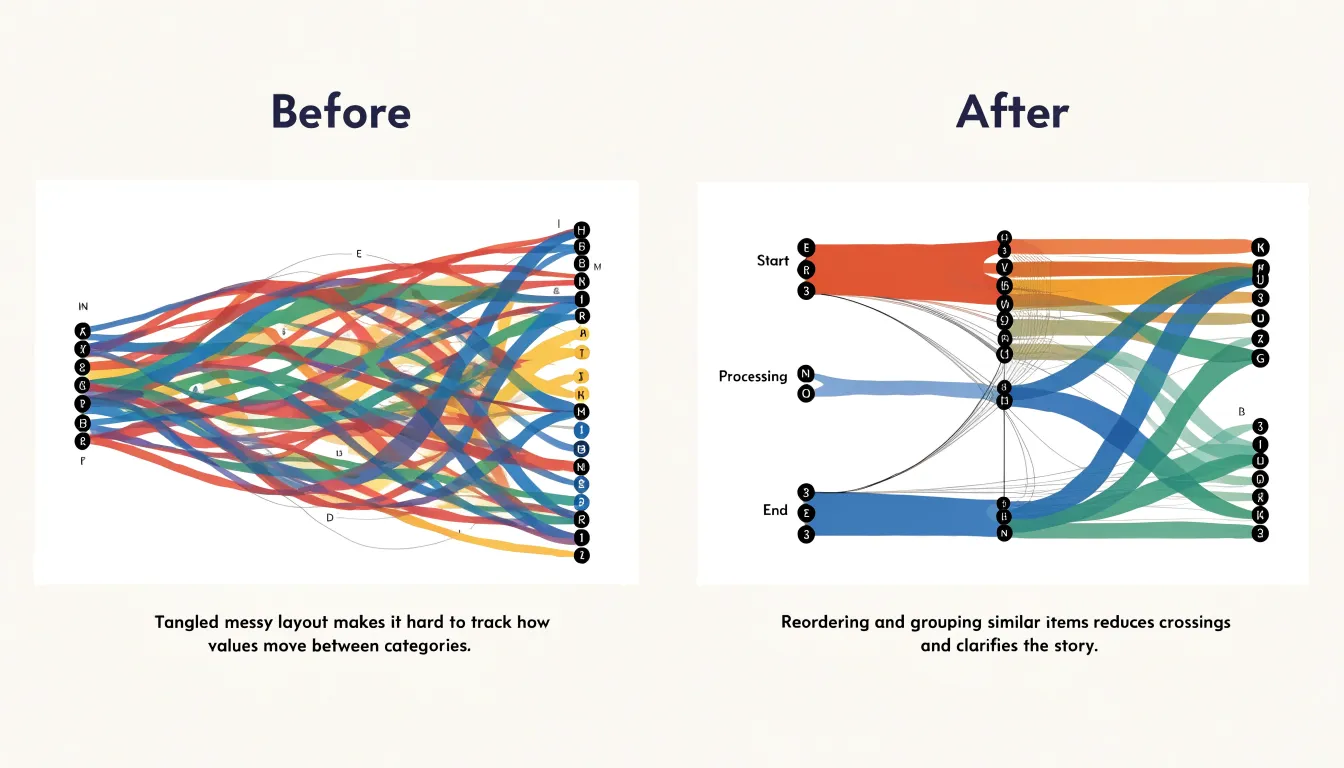
The underlying principle across all three pitfalls is restraint: every added link, node, and crossing carries a cognitive cost, and the diagram works best when designers prioritize clarity over completeness.
Color Coding
Color coding in Sankey and alluvial diagrams guides the eye toward the flows that matter most. One effective technique is the strategic use of gradient transitions along each link, letting color shift from the source node’s hue to the target node’s hue across the ribbon’s length. Gradients communicate direction and continuity at a glance, so viewers can trace a flow from origin to destination without consulting a legend.
A related approach is source-node hue inheritance, where every outgoing link adopts the color of its originating node and holds it steadily along the path. This makes it easy to see which source generated a given stream and to follow intertwined ribbons back to their common origin, which is especially valuable in dense diagrams with many crossing links.
Highlight colors add a further layer of emphasis. Designers often render the bulk of the diagram in muted, low-saturation tones and reserve a single saturated accent for the critical pathway under discussion. That contrast draws attention instantly in presentations where one message must dominate. Highlight colors can also mark exceptions—such as anomalous flows, losses, or leakage between stages—using a distinct hue that separates them from routine traffic.
When combining gradients, inheritance, and highlights, consistency matters: a small palette of well-chosen hues, applied with a clear rule about when each technique is used, keeps the diagram readable. Testing the palette for color-vision accessibility and sufficient lightness differences between adjacent ribbons protects legibility.
Data Preparation
Both Sankey and alluvial diagrams rely on the same underlying data structure: a set of nodes connected by weighted links. The most common starting point is a row-based table containing three columns—source, target, and value. Each row represents one flow, naming the origin node, the destination node, and the magnitude of the flow. Check that every node name appears in both the source and target columns where relevant, that numeric values are stored as numbers rather than strings, and that there are no duplicate rows covering the same connection unless you intend to sum them during aggregation.
Beyond the tabular form, many libraries expect a node-link JSON structure. In D3.js, the sankey layout typically takes an object with a nodes array and a links array. Each node entry has a name or id field, and each link entry has source, target, and value fields. Depending on the D3 version, the source and target can be provided as names or numeric indices that reference positions in the nodes array. Python libraries such as Plotly, HoloViews, and pySankey have their own conventions: some accept the source-target-value DataFrame directly, while others require separate node and link collections. Reading the documentation for your chosen tool before building the JSON avoids repeated restructuring.
Validation saves time downstream. Confirm that every source and target in the link set corresponds to a declared node, that values are non-negative, and that the data is free of cycles if the layout cannot handle them. Sorting nodes into a logical order and grouping them by category or stage also helps the renderer produce a readable layout.
Reading Dense Graphs
Dense diagrams reward a structured reading strategy:
- Begin with the largest flows and work outward. The thickest bands carry the primary story, so trace each major flow from its source node through every intermediate stage to its final destination. Note the relative width at each stage, since a band that narrows sharply signals significant loss or conversion along that path. Once the dominant flows are mapped, move to the mid-sized bands and then to the thin filaments, which often reveal secondary patterns such as leakage, residual categories, or minority pathways.
- Work systematically through the node columns. Rather than jumping between columns, count how many links enter and leave each node, and observe whether the totals balance at each stage. Imbalances frequently indicate aggregation choices, omitted categories, or data quality issues worth flagging. Tracing one path at a time across every column helps build an accurate mental model of how individual units travel through the system.
- Check color and grouping conventions. Verify in the legend whether colors represent sources, destinations, or intermediate states. Where colors repeat across columns, the diagram is likely tracking continuity of the same category through multiple stages. Interactive versions often allow hovering to isolate a single path; static readers can simulate this by physically tracing bands with a finger or cursor.
- Use simplification tactics when overwhelmed. Filter out categories below a threshold, collapse minor nodes into an “other” group, or re-sort nodes by magnitude rather than alphabetically. Compare a simplified view against the full diagram to confirm that it preserves the essential structure, then return to the detailed version with a clearer map of what matters.
Case Studies
Real-world applications demonstrate how Sankey and alluvial diagrams serve distinct analytical purposes in logistics and demography.
In supply chain management, a global electronics manufacturer mapped its end-to-end logistics network using a Sankey diagram to visualize the flow of components from suppliers to assembly plants and distribution centers. The width-proportional links revealed bottlenecks at specific transshipment hubs, where material volume exceeded capacity and caused delays. By adjusting flows and rerouting shipments, the company reduced lead times by 15%. The Sankey diagram’s conservation of flow made it ideal for tracking physical goods and identifying inefficiencies.
For demographic analysis, a longitudinal study of internal migration patterns in a rapidly urbanizing region employed an alluvial diagram to track population movements over three decades. The alluvial structure displayed how cohorts moved between rural, peri-urban, and urban categories across census years. This revealed a steady drift toward metropolitan areas, with a notable counter-flow of retirees to rural destinations after 2010. The diagram’s strength lay in showing changes in categorical composition over time, allowing researchers to observe both stable and shifting migration streams.
Choosing the Right Chart
To select between a Sankey diagram and an alluvial diagram, evaluate the underlying data using this three-step checklist:
- Check for conserved quantities. Ask whether your dataset describes conserved quantities flowing between states, such as energy, money, or material volumes, where the total entering a node should equal the total leaving it. Non-conserved data may call for a different chart family entirely, or a non-conservative alluvial layout.
- Check for a time dimension. Alluvial diagrams are built to show how categories shift across ordered stages or periods, so a dataset with multiple snapshots, cohort movements, or sequential stages points toward an alluvial layout. Sankey diagrams work well for a single integrated flow picture at one point in time without a strict temporal backbone.
- Assess dataset dimensionality. Count the number of categorical dimensions and flow layers. A simple source-to-target flow with a few intermediate nodes fits a Sankey diagram cleanly. Data with several categorical strata that persist across stages, where each stratum carries an identity from beginning to end, benefits from the alluvial structure that keeps those strands visually traceable.
When the sequence is temporal and strata must remain identifiable across stages, choose the alluvial diagram. When the priority is a clear picture of aggregate, conserved flows through a network, choose the Sankey diagram.
Overview
Interactive features transform static flow diagrams into exploratory tools for web-based dashboards:
- Tooltips: Hovering over a node or link reveals precise values, labels, and contextual details. This on-demand access keeps the main view uncluttered while supporting deeper inquiry, letting viewers move fluidly between a system overview and the specifics of a single flow.
- Node highlighting: Selecting a particular category highlights every connection related to it while dimming unrelated elements. This visual focus helps users trace relationships across dense networks without losing their place and makes comparing competing pathways easier.
- Path dragging: Users can reposition nodes or drag along a flow path to follow a quantity from its origin through intermediate stages to its destination, supporting a clearer understanding of how resources, energy, or value move through a system.
- Dynamic filtering: Viewers can narrow the displayed data according to thresholds, time periods, or categories, adapting the visualization to different analytical needs.
Together, these features lower the barrier to entry for non-specialist audiences while offering depth for expert users, turning flow diagrams into decision-support tools where users can test scenarios and isolate problem areas.
Frequently Asked Questions
What is the difference between a Sankey diagram and an alluvial diagram?
A Sankey diagram represents conservative transfer systems where the total quantity of a resource remains constant as it moves between stages, with inflows balancing outflows at each node. An alluvial diagram traces groups or clusters as they persist, split, merge, or dissolve across a sequence of time steps or processing stages, and it can allow non-conservative flows.
What do flow widths represent in Sankey and alluvial diagrams?
Flow widths are the primary visual encoding in both diagram types, and the thickness of each link represents a scalar quantity such as energy, money, or people. When widths are strictly proportional, a link twice as thick as another represents twice the quantity.
When should I use an alluvial diagram instead of a Sankey diagram?
Use an alluvial diagram when the sequence is temporal and strata must remain identifiable across stages, or when the data has multiple snapshots, cohort movements, or sequential stages. Use a Sankey diagram when the priority is a clear picture of aggregate, conserved flows through a network.
What data structure do Sankey and alluvial diagrams need?
Both diagram types rely on a set of nodes connected by weighted links, and a common starting point is a row-based table with source, target, and value columns. Many libraries expect a node-link JSON structure with nodes and links arrays, and validation should confirm that every source and target corresponds to a declared node, values are non-negative, and the data is free of cycles if the layout cannot handle them.
What are common design pitfalls in Sankey and alluvial diagrams?
Common pitfalls include excessive line crossing, unreadable small links, and over-segmentation. The article recommends careful node ordering, applying a minimum thickness or aggregating negligible flows, and consolidating fine-grained categories or limiting stages to keep the diagram clear.
How should I read a dense Sankey or alluvial diagram?
Begin with the largest flows and work outward, then work systematically through the node columns and check color and grouping conventions. When overwhelmed, filter out categories below a threshold, collapse minor nodes into an “other” group, or re-sort nodes by magnitude rather than alphabetically.
Tony Astor
Tony writes about data visualization and the tools people use to build charts and dashboards. More about Data Illustrator