Ridgeline Plot vs Histogram: Comparing Distributions
 By Tony Astor ·
Ridgeline Plot vs Histogram
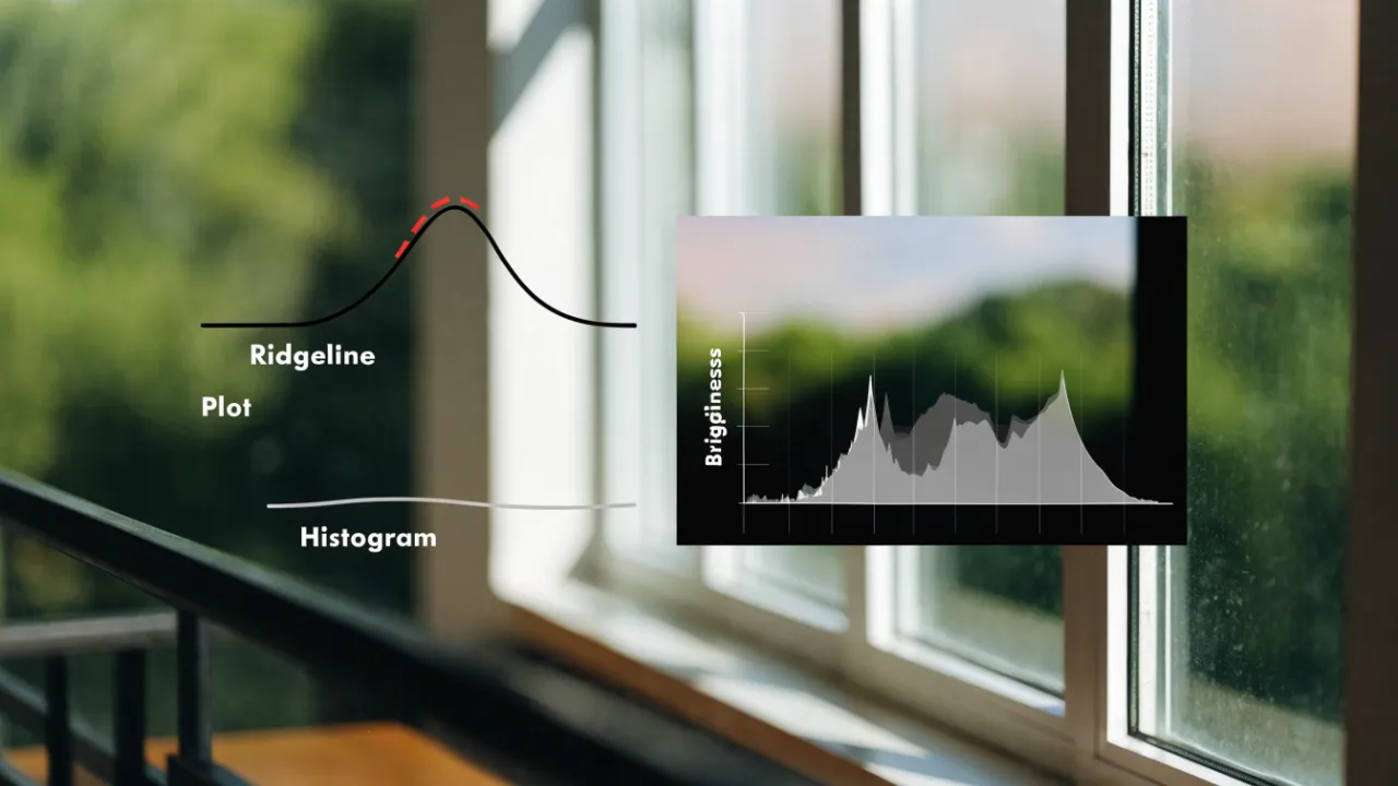
A ridgeline plot stacks kernel density curves for many groups on a shared axis, making it ideal for comparing dozens of distributions; a histogram bins one variable’s values into adjacent bars showing exact counts, making it the clearest choice for single-group analysis. Choose ridgelines for many groups or time series, histograms for one dataset.
Table of Contents
Histogram
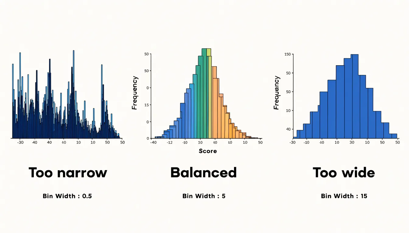
A histogram takes a continuous numeric variable and slices its range into a series of adjacent intervals, usually called bins, then counts how many observations fall into each one. The horizontal axis represents the measured values, divided into these intervals, while the vertical axis records the number of observations, or frequency, within each interval. Bars are drawn side by side with no gap between them, which visually signals that the underlying variable is continuous and that each bin flows directly into the next. The choice of bin width shapes what the reader sees: narrow bins expose fine-grained detail and local spikes, while wider bins smooth those details away and reveal the broader structure of the distribution.
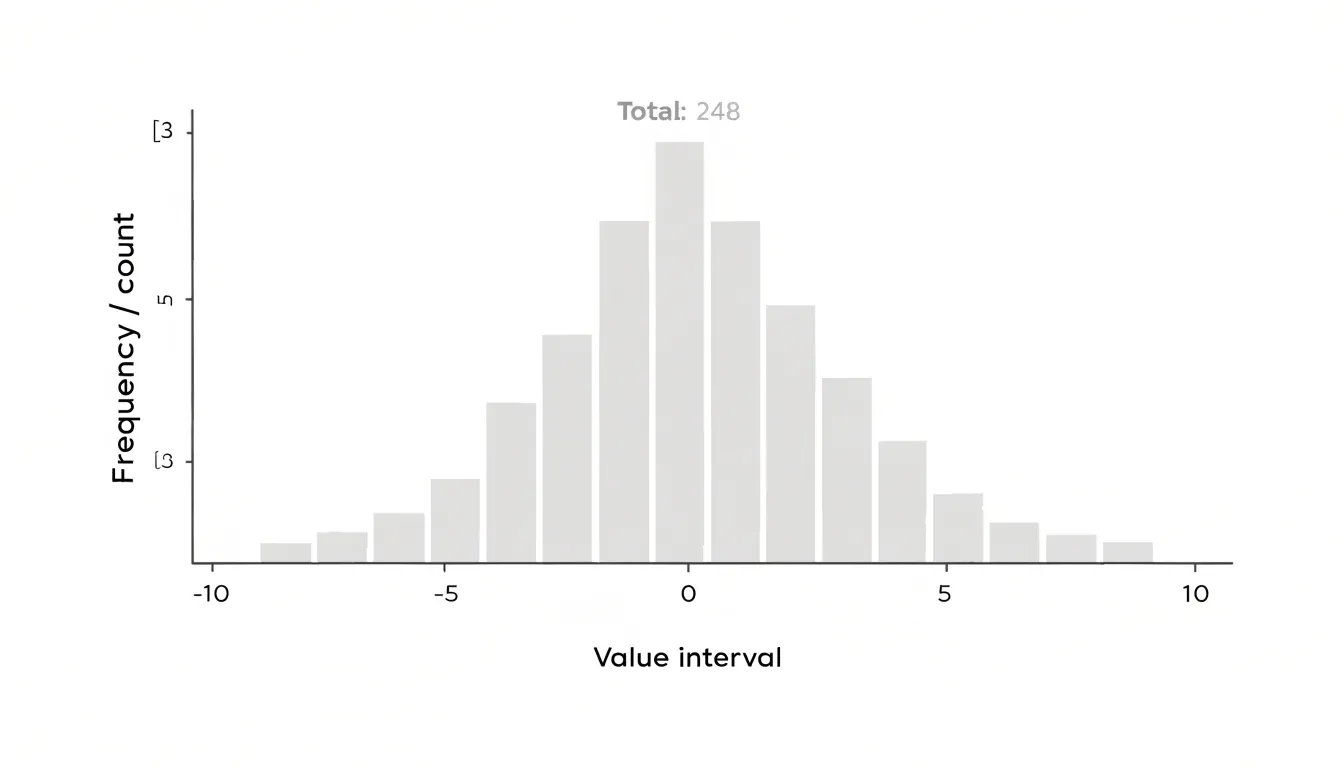
Because every observation is assigned to exactly one bin, the histogram summarizes the full dataset in a single view. The resulting outline of bar heights shows the shape of the distribution, including where values cluster, where the data thins out, and whether the pattern is roughly symmetric or skewed toward one side. Peaks in the outline point to common values, and long tails point to rarer extremes. The total area of the bars corresponds to the total number of observations, so relative frequencies can be read directly from bar heights when all bins share the same width.
Histograms work best for a single variable at a time, and their appearance depends on decisions made during construction, especially bin count and bin boundaries. Shifting the starting point of the bins can change the visual pattern even when the data stay the same. This makes the histogram a flexible and widely used first step in exploratory analysis, offering a compact picture of frequency counts and overall shape across one dataset before more detailed comparisons are attempted.
Ridgeline Plot
A ridgeline plot arranges a series of kernel density estimates as stacked, partially overlapping curves along a single shared horizontal axis, with each curve corresponding to one category or group. Rather than placing every distribution in its own panel, the ridgeline plot offsets each density vertically by a small, consistent amount so that the curves overlap just enough to stay visually connected while remaining individually readable. The result is a compact visual stack in which the shape, central tendency, spread, and skew of dozens of distributions can be scanned in a single pass.
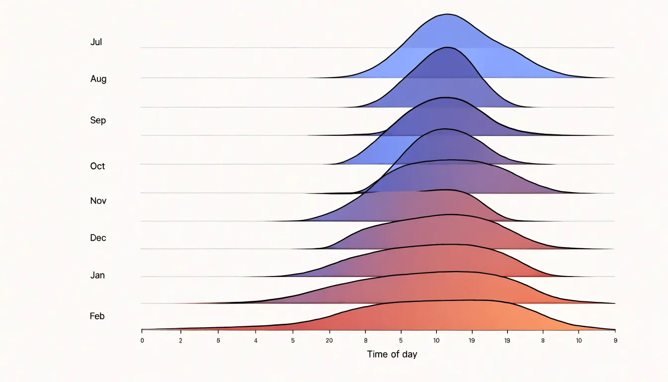
Each row typically represents a group, such as a month, a region, or a category in a dataset, and the horizontal position encodes the value being measured. The vertical offset provides separation without introducing a second quantitative axis, so the reader’s eye moves naturally down the stack, comparing peaks, tails, and shoulders across adjacent rows. Because the densities are estimated from the underlying data using kernel density estimation, the curves smooth out the noise of raw observations and reveal the overall contour of each group’s distribution.
The partial overlap is central to the design. Full separation would turn the figure into a grid of disconnected mini-charts, while complete overlap would obscure individual shapes. By allowing successive curves to touch and slightly interleave, the ridgeline plot creates a continuous visual rhythm that draws the eye along the sequence of groups and makes it easy to spot trends, such as a distribution shifting gradually toward higher values over time or a subgroup developing a distinctive secondary peak. This makes the format well suited to comparing many categories at once, particularly when the interest lies in how distributions change across an ordered dimension rather than in precise point estimates.
Single Group Analysis
A standalone histogram remains the clearest tool for inspecting one variable on its own. When the analytical question concerns a single group, the histogram answers it directly: each bar shows the raw count of observations falling within a defined bin, so the viewer reads exact frequencies straight from the bar heights. That simplicity carries real analytical value. There is no layering, no overlapping series, and no need to decode which color or curve belongs to which category, which means attention stays entirely on the shape and substance of the distribution.
The granular bin structure is another strength in single-group settings. Analysts can tune bin width to reveal fine detail such as gaps, spikes, or clustering that might be smoothed over by density estimation or obscured by multiple overlaid curves. Because every observation contributes to exactly one bar, the histogram preserves an honest accounting of the data, and the total of the bar heights equals the sample size. This makes it easy to verify counts, spot unusual concentrations, and communicate findings to audiences who need exact numbers rather than an impression of shape.
Speed of construction also matters. A basic histogram requires only the variable itself and a reasonable choice of bin count, making it a natural first step in exploratory analysis before any more elaborate visualization is considered. It serves as a stable reference point that later, richer plots can be compared against. When the goal is to understand one variable thoroughly, the standalone histogram offers completeness without added complexity, and that combination keeps it the default choice for single-group inspection.
Multiple Datasets
When comparing multiple datasets, a ridgeline plot offers a clear advantage by stacking density curves vertically, each with a slight overlap that creates a smooth, continuous visual flow. This arrangement prevents the visual clutter that arises when trying to layer multiple histograms on the same set of axes. Histograms, by nature, are blocky and space-filling; overlaying several of them forces the viewer to decipher which bars belong to which dataset, especially when distributions overlap. The result is a tangled mess of colors and heights that obscures patterns and makes comparisons difficult.
Ridgeline plots sidestep this problem by giving each dataset its own horizontal baseline, offset vertically. The curves are drawn as filled densities, and the slight overlap between adjacent ridges creates a sense of depth without sacrificing clarity. Each distribution remains distinct, yet the eye can easily trace the shape of each curve and compare features like peaks, spread, and skewness across datasets. This layout is particularly effective when dealing with many groups, as it avoids the crowding that would occur if all histograms were superimposed.
Moreover, the stacked arrangement allows for a natural ordering—often by median or another summary statistic—which further aids comparison. Viewers can quickly scan from top to bottom and see how distributions shift. The use of transparency or subtle color variations enhances the effect, making overlaps visible without confusion. In contrast, layered histograms with transparency often produce muddy colors where bars intersect, and the additive nature of bar heights can mislead about density.
By preventing heavy overlap and visual clutter, ridgeline plots make it easier to discern subtle differences between datasets. They leverage the human visual system’s ability to compare shapes along a common axis, turning a potentially chaotic comparison into an orderly and informative display.
Time Series
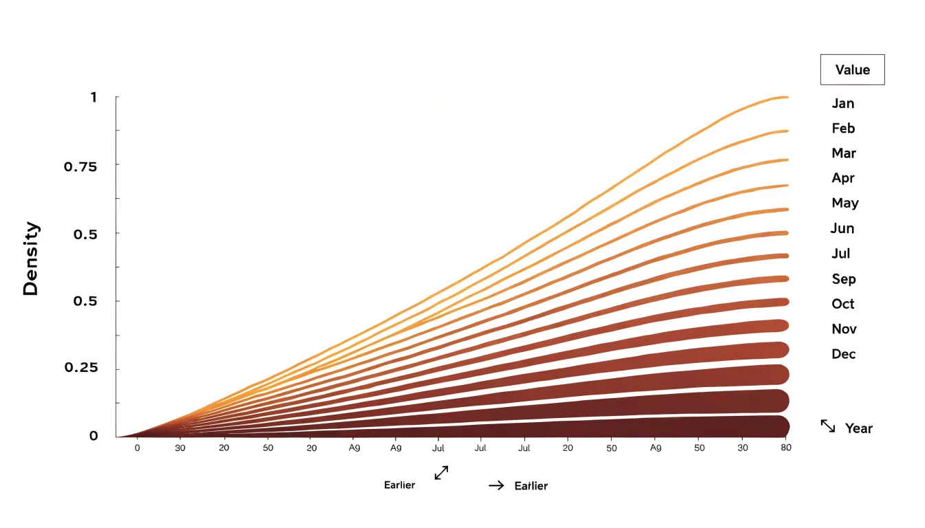
When a dataset carries a temporal dimension, the arrangement of its visual elements becomes a meaningful part of the analysis. A ridgeline plot stacks one density curve per time period, such as a month or a year, along a shared horizontal axis, and ordering those curves chronologically turns the display into a narrative of change. Each row preserves the full shape of a distribution for its period, so the reader can follow the movement of peaks, the widening or narrowing of spread, and the emergence of secondary modes from one period to the next. This chronological ordering is what allows subtle evolutionary trends to surface. A gradual shift in the central tendency, for instance, appears as a slow diagonal drift across the stack rather than as a single dramatic jump, and that gentle migration is easy to miss in isolated per-period charts. Seasonal shifts likewise become visible as recurring patterns of expansion and contraction, where certain months consistently produce broader or more skewed distributions while others remain tight and centered. Distribution drift, the slow reshaping of a population over years, shows up as a progressive change in the silhouette of successive ridges, whether through the thinning of tails, the smoothing of multimodal shapes, or the creeping ascent of a formerly minor peak. By placing periods in sequence and sharing a common scale, the ridgeline plot lets these movements be compared directly, with earlier distributions remaining in view as context for later ones. The result is a compact visual record of how a quantity evolves, where the vertical rhythm of the ridges encodes time and the contours of each curve encode the changing shape of the underlying data.
Reading Density Curves
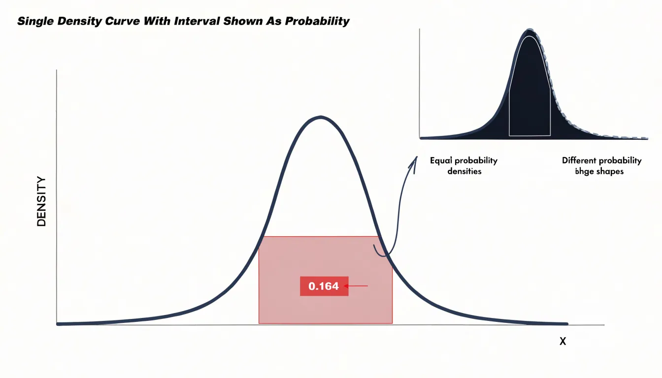
Reading Density Curves — understanding smooth waves instead of bars: A density curve replaces the familiar stack of histogram bars with a smooth, continuous wave, and learning to read it correctly changes how you extract meaning from a distribution. The curve is typically produced through kernel density estimation, a procedure that places a small bump, called a kernel, at the location of every data point and then sums those bumps together. Where observations cluster closely, the individual kernels overlap and accumulate, producing a tall peak; where observations are sparse, the bumps spread thin and the curve stays low. The bandwidth setting controls how wide each kernel spreads, so a narrow bandwidth yields a jagged curve that follows every data point, while a wide bandwidth yields a gently rolling curve that reveals the broader shape. This is why the curve is described as a wave rather than a bar chart: it flows across the entire number line and never breaks into discrete steps.
The most important skill in reading these curves is focusing on area rather than height. In a histogram, the height of a bar corresponds directly to the count of observations in that bin, so taller means more. In a density curve, height is only meaningful in relation to the width of the region beneath it. The probability of values falling within any interval is the area under the curve across that interval, and the total area beneath the entire curve equals one. A tall, narrow peak and a low, broad hump can enclose exactly the same area, and therefore represent the same amount of probability. Practitioners who read raw heights as if they were frequencies will misjudge how much data sits in a region, especially when comparing distributions with different spreads. The reliable habit is to estimate areas over intervals of interest, look for where the curve encloses the most region, and treat the smooth shape as a summary of density that spreads probability across the full range of values.
Bin Widths
Bin widths determine how a histogram communicates the shape of a distribution. Every value in a dataset falls into a bin, and the width of those bins sets the resolution at which patterns become visible. When bins are too narrow, each bar captures only a handful of observations, and the resulting chart fills with jagged spikes and gaps that reflect sampling noise rather than underlying structure. A reader may mistake these fluctuations for real features, such as secondary peaks or clusters, when they are simply artifacts of an overly fine partition. Over-binning also multiplies the number of bars, cluttering the axis and making comparisons between groups harder to follow.
At the opposite extreme, wide bins merge distinct features into single blocks. A bimodal distribution can collapse into one broad mound, and a subtle skew or outlier region can disappear entirely. Under-binning smooths away the detail that makes a histogram useful, trading noise for a loss of information. The practical challenge lies in finding a width that preserves meaningful structure while suppressing random variation.
Several rules of thumb offer starting points. Sturges’ rule works well for small, roughly normal samples, while Freedman-Diaconis adjusts for spread and sample size and performs better with skewed or heavy-tailed data. Scott’s rule provides another balanced default. These formulas give a reasonable first guess, yet the final choice often benefits from testing a few widths side by side and checking which features persist across them. Features that remain stable as bin width changes are likely real; those that appear and vanish are probably noise. Adjusting the starting point of bins can also reveal whether apparent patterns depend on arbitrary boundaries. With careful selection, the histogram becomes a reliable portrait of the distribution rather than a reflection of arbitrary chart settings.
Smoothing Factors
Smoothing factors in ridgeline plots determine how curve settings shape the density estimates. The key parameter is the bandwidth of the kernel density estimator, which controls the width of the smoothing kernel applied to each data point. A small bandwidth produces a spiky curve that follows every fluctuation in the sample, including random noise. This under-smoothing can obscure the overall distribution by highlighting irrelevant variations. Conversely, a large bandwidth yields a very smooth curve that may merge distinct peaks and hide meaningful structure, a problem known as over-smoothing. The choice of bandwidth thus involves a trade-off between bias and variance. Automated methods like Silverman’s rule of thumb or cross-validation provide starting points, but the appropriate bandwidth often depends on the data and the story you want to tell. In ridgeline plots, where multiple distributions are stacked for comparison, consistent bandwidth across groups is essential for fair visual comparison. Varying bandwidth between groups can create misleading impressions of differences in spread or modality. Additionally, the kernel shape (e.g., Gaussian, Epanechnikov) affects the smoothness, though bandwidth has a larger impact. When adjusting smoothing, it’s helpful to view the plot at multiple bandwidths to see which features are robust. Peaks that persist across a range of bandwidths are likely real, while those that appear only at very low bandwidths may be noise. Ultimately, the goal is to choose a smoothing level that reveals the underlying structure without imposing artifacts, balancing clarity and fidelity to the data.
Overlapping Areas
When comparing closely matched cohorts, the challenge lies in detecting subtle differences that might otherwise go unnoticed. Overlapping areas in a ridgeline plot offer a powerful solution by leveraging translucency and stacked ridge positioning. Translucency allows multiple distributions to be overlaid, so that regions of overlap remain visible while each group’s density curve is still distinguishable. This is particularly useful for revealing subtle mean shifts: even a slight displacement between two similar distributions becomes apparent when their semi-transparent areas partially cover each other, creating a visual gradient that highlights the divergence. Similarly, changes in variance are easier to spot; a group with slightly wider spread will show a broader, more diffuse overlapping area, while a narrower distribution will appear more concentrated. Multimodal distributions, which might be obscured in a standard histogram due to binning artifacts or aggregation, are also more evident in a ridgeline plot because each mode appears as a distinct peak within the translucent area, and overlapping modes from different groups can be compared directly. Stacked ridge positioning further enhances these comparisons by aligning distributions along a common baseline, with each group offset vertically. This arrangement allows viewers to scan across groups and quickly assess differences in central tendency, spread, and shape without the visual clutter of overlapping histograms. The combination of translucency and stacking creates a layered effect where subtle variations emerge naturally, making ridgeline plots particularly effective for exploratory analysis of closely matched cohorts, such as treatment vs. control groups or demographic subgroups, where small but meaningful differences can have important implications.
Space Efficiency
Ridgeline plots are built around the principle of overlapping density curves that share a common horizontal axis while each category receives its own compact band of vertical space. The savings come from the way adjacent curves are allowed to overlap slightly, so the baseline of one ridge sits just above the peak region of the ridge beneath it. This arrangement compresses what would otherwise be a full panel per category into a thin slice, and the partial overlap means the eye still reads each distribution clearly without the chart demanding a separate row of equal height.
Consider evaluating several dozen categories at once. A grid of faceted small multiples allocates a complete panel to each category, complete with its own axis, labels, and whitespace. With forty categories arranged in a sensible grid, each panel shrinks until the curves inside become tiny and hard to compare, or the figure grows to the point where it no longer fits comfortably on a page or screen. Side-by-side boxplots face a similar constraint in the opposite orientation. Placing dozens of boxes along a single horizontal axis forces either a very wide figure or heavily crowded, overlapping labels beneath every box.
The ridgeline layout resolves this by stacking categories vertically and letting the density shapes do the work of separating them. A single shared x-axis at the bottom serves every ridge, so no vertical space is spent repeating tick marks and axis labels. Category labels sit to the left of each ridge, aligned in a tidy column, which keeps the plot readable even at high category counts. The result is a chart that can display thirty, fifty, or more distributions in a figure roughly the height of a standard slide, making efficient use of vertical canvas while preserving enough detail in each curve to compare shapes, peaks, and spread across the full set of categories.
Skewness and Outliers
Skewness describes the asymmetry of a distribution, and both histograms and ridgeline plots make that asymmetry visible in different ways. A histogram shows skew through the shape of its bars: a positive skew produces a tall cluster of bars on the left with progressively shorter bars trailing off to the right, while a negative skew mirrors this pattern with the long tail extending leftward. The eye reads the imbalance immediately, noting where the mass of observations sits relative to the stretched-out side of the distribution. Ridgeline plots carry the same information through density curves, where skew appears as a lopsided peak with one side descending gradually while the other drops steeply. Because ridgelines stack multiple distributions vertically, comparing skew across groups becomes a matter of scanning the outlines and noticing which rows lean left or right.
Long tails deserve close attention in either format. In a histogram, a long tail shows up as a thin scattering of short bars stretching away from the main body, sometimes so sparse that individual counts are hard to read. In a ridgeline, the tail is a thin filament of density that tapers toward the axis, and slight bumps along that taper can reveal small clusters of unusual values. Extreme values are the points furthest along these tails, and they influence summary statistics such as the mean, pulling it toward the tail and away from the median.
Identifying outliers visually means looking for bars that stand isolated from the main cluster or density bumps that rise unexpectedly far from the central peak. These features sometimes signal genuine rare events and sometimes point to data entry errors, so flagging them is a first step toward investigation. Practically, zooming into tail regions, annotating the axis range, and comparing summary statistics alongside the visual shape all help turn a quick impression of skewness into a reliable reading of the distribution’s behavior.
Large Datasets
As sample sizes climb into the tens of thousands or millions, a histogram’s fixed number of bins becomes a limitation: each bar aggregates so many observations that the shape blurs into a handful of coarse blocks, and the individual structure that made the data interesting disappears. Increasing the bin count to compensate introduces a different problem, since narrow bins produce a jagged, noisy profile that changes shape dramatically depending on where the bin edges happen to fall. A ridgeline plot sidesteps this tradeoff by representing each distribution as a smooth density curve, so the visual mass of the data is preserved even when millions of points contribute to a single shape. The curve adapts to the underlying sample, capturing fine structure such as secondary peaks or long tails without demanding a manual choice of bin width. When multiple groups are stacked along the vertical axis, the reader can scan dozens of distributions at once and immediately see which categories shift, widen, or develop additional modes over the range being displayed. The overlapping, offset layout also prevents the crowding that occurs when many histograms are drawn on shared axes, because each ridge occupies its own baseline while still allowing direct comparison of density height and spread. This makes ridgeline plots particularly effective for large collections of mass data, such as daily readings across a year or measurements across many categories, where the goal is to spot broad trends and outliers at a glance. The visual encoding remains legible as the dataset grows, keeping the overall pattern readable while still reflecting the weight of the underlying observations.
Common Pitfalls
When constructing a ridgeline plot, several common pitfalls can undermine the clarity and accuracy of the visualization. One frequent error is truncating the baseline of the density curves, which can exaggerate small differences and make distributions appear more distinct than they are. Always start the y-axis at zero for each density estimate to maintain proportional representation. Another key mistake is choosing bin widths or bandwidths that are too large or too small. Overly wide bins smooth out important features, while narrow bins introduce noise and spurious peaks. Experiment with multiple settings and consider using cross-validation to select an appropriate bandwidth. A third pitfall is allowing heavy overlap between ridges, which can obscure shorter background distributions. While some overlap is inherent to the ridgeline design, excessive overlap can hide peaks entirely. Adjust the vertical spacing between ridges or use transparency to ensure all distributions remain visible. Additionally, be cautious with color choices; using similar colors for adjacent ridges can make them blend together. Instead, use a sequential palette or vary lightness to distinguish groups. Finally, avoid overplotting too many ridges in a single plot, as this can lead to visual clutter. If necessary, split the data into multiple panels or use faceting. By addressing these pitfalls, you can create ridgeline plots that are both informative and visually appealing, accurately conveying the structure of your data without misleading the viewer.
Selection Strategy
A decision framework for choosing between histograms and ridgeline plots rests on four practical inputs: sample size, the number of groups, the target audience, and the output medium. Each input points toward one chart or the other with reasonable consistency, and working through them in order takes only a moment.
Sample size sets the foundation. With a single modest dataset, a histogram gives a clear, honest picture of the distribution’s shape, center, and spread. As observations accumulate per group, a histogram remains workable, but the density detail it reveals becomes richer and more trustworthy for comparison across categories. A ridgeline plot earns its place when each group contains enough observations for a smooth density estimate, since sparse groups produce jagged curves that exaggerate noise.
The number of groups is the second consideration. A handful of distributions sit comfortably side by side as small-multiple histograms, where each panel stays legible. Once the group count climbs into the dozens, stacking histograms becomes unwieldy, and the ridge layout’s shared axis and vertical offsets keep every distribution visible in a compact band. Ridgelines scale gracefully in this direction, while histograms fragment the page.
Audience shapes the choice further. Readers with statistical training read overlapping densities without difficulty. A general audience responds better to familiar bars, so a histogram or a small set of histograms reduces interpretive friction.
Finally, the output medium matters. Print and static reports favor whichever chart stays readable at the intended size, and ridgelines compress many groups into a narrow column without losing detail. Interactive dashboards reward histograms linked to filters and tooltips, where users can drill into individual groups.
Weighing these four inputs together yields a defensible chart choice every time.
Frequently Asked Questions
What is the difference between a histogram and a ridgeline plot?
A histogram divides a continuous numeric variable into adjacent bins and counts how many observations fall into each one, drawing bars side by side with no gaps. A ridgeline plot stacks kernel density estimates for categories or groups as partially overlapping curves along a shared horizontal axis.
When is a histogram better than a ridgeline plot?
A standalone histogram is the clearest tool for inspecting one variable or a single group, because each bar shows the raw count of observations in a bin. It avoids layering and overlapping series, so attention stays on the shape and substance of the distribution.
How do bin widths affect a histogram?
Bin widths control the resolution of a histogram: narrow bins expose fine-grained detail and local spikes but can reflect sampling noise, while wider bins smooth details away and reveal broader structure. Choosing a width involves preserving meaningful structure while suppressing random variation, and testing several widths helps show which features are stable.
Why use a ridgeline plot for comparing multiple datasets?
A ridgeline plot stacks density curves vertically with slight overlap, which prevents the visual clutter that arises when multiple histograms are layered on the same axes. Each distribution remains distinct while the eye can compare features like peaks, spread, and skewness across datasets.
How do you read a density curve in a ridgeline plot?
In a density curve, focus on area rather than raw height: the probability of values falling within an interval is the area under the curve across that interval, and the total area beneath the entire curve equals one. A tall, narrow peak and a low, broad hump can enclose the same area and represent the same amount of probability.
Can ridgeline plots show changes over time?
Yes, a ridgeline plot can stack one density curve per time period along a shared horizontal axis and order those curves chronologically. This arrangement makes gradual shifts in central tendency, seasonal patterns, and distribution drift visible across periods.
Tony Astor
Tony writes about data visualization and the tools people use to build charts and dashboards. More about Data Illustrator