Ridgeline Plot: Comparing Many Distributions at Once
 By Tony Astor ·

Ridgeline Plot
A ridgeline plot stacks many density curves or histograms vertically, with each row representing a distinct group and all rows sharing one horizontal scale for the measured variable. Overlapping curves rise from offset baselines, letting viewers compare peaks, spread, skew, and multimodality across dozens of distributions in a compact space.
Table of Contents
Ridgeline Plot
A ridgeline plot arranges many density curves or histograms in a vertical stack, with each row corresponding to a distinct group, category, or time period. The horizontal axis carries the quantitative variable being compared, so every row shares the same measurement scale along the bottom of the chart. This shared scale is what makes the display useful: a peak, a long tail, or a bimodal shape in one row can be compared directly against the rows above and below it, because a given horizontal position refers to the same value everywhere in the figure.
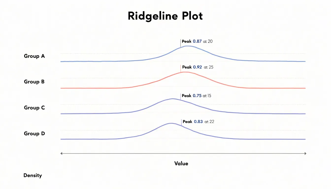
The vertical dimension works differently. Each group gets its own baseline axis, drawn as a horizontal line at that group’s position in the stack. The curves rise from these baselines rather than from a single shared zero line, which means the vertical extent of a curve encodes density or frequency within its row, while the row’s position encodes group membership. Readers move down the stack to scan across groups and move left to right to read values along the shared quantitative axis. Labels on the left, or sometimes on each baseline, identify which group each row represents.
Because the baselines are offset and the curves often overlap slightly with their neighbors, the chart compresses a large number of distributions into a compact space without the clutter of dozens of separate small charts. The overlapping creates a layered, mountainous appearance, which is where the name comes from. To read one, start by locating the group labels and confirming the order of the stack, then trace each row’s curve from its baseline upward to see where its mass concentrates. Comparing the horizontal position of peaks across rows reveals shifts in typical values, while comparing curve widths and tail lengths reveals changes in spread or the appearance of secondary clusters.
Density Curves
Each curve in a ridgeline plot represents a probability density estimate for one category, and interpreting these curves begins with understanding what the shape reveals. The peak of a density curve indicates the most probable value or the mode of the distribution—where observations are most concentrated. A sharp, narrow peak suggests that values cluster tightly around that point, implying low variability. In contrast, a broad, flat peak indicates that the data are more spread out, with a wider range of typical values. The height of the peak also matters: a taller peak means a higher density at that point, which often corresponds to a larger number of observations in that region relative to the total. However, because density curves are scaled to integrate to one, comparing peak heights across curves can reveal differences in concentration even when sample sizes vary.
Spread, or dispersion, describes how wide the distribution is. A curve that stretches over a large range on the x-axis indicates high variability, while a compressed curve suggests homogeneity. The width at half the peak’s height (full width at half maximum) provides a useful summary of spread. Tail thickness is another critical feature: heavy tails indicate a higher probability of extreme values, meaning outliers are more likely. Light tails suggest that extreme values are rare. By examining the tails, you can assess the risk of unusual observations within each category.
Interpreting these features together allows you to compare distributions effectively. For instance, two categories might have similar peaks but differ in tail behavior, signaling different risks of extreme outcomes. Ridgeline plots make these comparisons intuitive by stacking curves, so you can quickly scan for differences in peak location, spread, and tail weight across categories. This visual summary of probability density helps in identifying patterns and anomalies that might be missed in summary statistics alone.
Stacking and Overlap
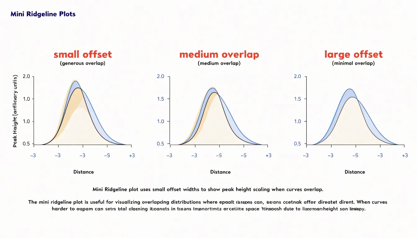
Layered ridgeline plots compress many distributions into a compact vertical band, and the spacing between rows determines whether the reader can compare trends cleanly or loses detail beneath overlapping shapes. The vertical offset assigned to each row sets a baseline for that distribution, while the overlap height controls how far each curve extends into the space of the row above it. Small offsets with generous overlap produce a dense, mountainous look that suits visual scanning of broad patterns, where the eye follows the crest line across categories. Larger offsets with reduced overlap give each distribution more breathing room, at the cost of a taller chart that consumes more vertical space on the page. A practical starting point is an overlap of roughly one half to two thirds of the row height, adjusted once the actual shapes are visible. Peak height matters as much as row spacing: a category with a tall sharp peak will cover the tail of the row behind it, so curving or scaling height or increasing the offset for that row protects the buried data. Transparency in the fill color helps where overlaps remain, letting shapes read through one another. Ordering rows by a meaningful statistic, such as median or peak position, keeps the stacking logic visible and makes comparisons follow a natural progression rather than an arbitrary sequence. When one row must sit above another to preserve the reading order, check that no distinct mode or shoulder in the lower curve disappears under the upper one. Baseline rules, a light horizontal line at each offset, anchor the eye to the row positions and clarify where one distribution ends and the next begins. Testing a few offset values against the real data, rather than fixing a default, usually reveals the setting where trends remain legible and detail survives.
Color and Gradients
Color serves as a powerful visual cue in ridgeline plots, guiding the eye to meaningful pattern changes across groups. By assigning distinct colors to each category or applying a continuous gradient along the x-axis, you can instantly highlight where distributions shift or cluster. For instance, a sequential palette that transitions from light to dark can emphasize increasing density, making high-density regions stand out without additional annotation. This approach is particularly effective when comparing many groups, as subtle changes in hue or saturation draw attention to differences that might otherwise go unnoticed.
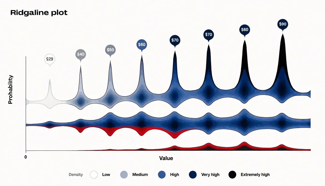
Heatmap-style coloring extends this idea by mapping density values directly to color intensity. In a ridgeline plot, this can be achieved by filling each ridge with a gradient that reflects the underlying density estimate, so peaks appear darker and valleys lighter. Such visual encoding allows viewers to quickly scan for multimodal distributions or overlapping clusters. When groups are ordered by a meaningful variable, a color gradient along the y-axis can further reveal trends, such as a gradual shift in distribution location or spread.
Fill gradients add another layer of nuance. By varying transparency or color along the fill, you can suggest uncertainty or highlight specific quantiles. For example, a gradient that fades toward the tails can draw focus to the central mass of each distribution. Combined with a thoughtful palette, these techniques transform a simple ridgeline plot into an informative visualization that communicates complex patterns at a glance. The key is to use color purposefully, ensuring that it enhances rather than distracts from the underlying data structure.
Distribution Shapes
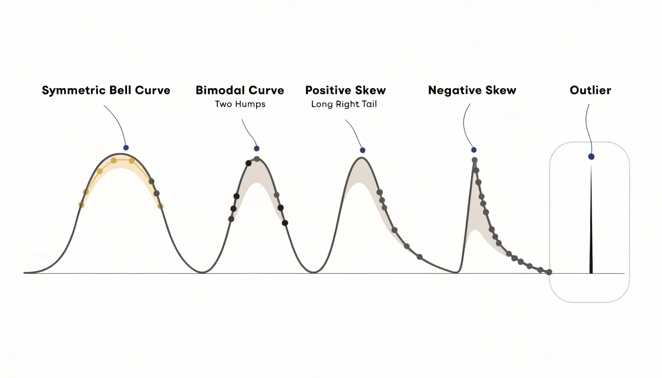
A ridgeline plot stacks many density curves along a shared axis, which makes it a natural instrument for comparing distribution shapes across dozens of groups. Once the curves are aligned, the eye can scan vertically and classify each group’s profile almost instantly. A symmetric, bell-shaped curve rising to a single central peak signals approximate normality: values cluster around a mean, and the tails taper evenly on both sides. When a curve swells across two distinct humps with a dip between them, the group is bimodal, hinting that two underlying populations or processes have been pooled together. A single long tail stretching toward the higher values marks positive skew, with most observations bunched at the low end and a few extreme high values pulling the mean up. Negative skew mirrors this, piling observations at the high end and trailing a thin tail toward lower values. Outliers appear as isolated bumps or thin spikes far along a tail, and because the plot shares a horizontal scale, these spikes line up against the corresponding positions in neighboring curves. The real payoff comes from density: stacked together, the curves let a reader check dozens of groups in a single glance, noticing which resemble the overall pattern, which deviate, and which shift location or spread relative to their neighbors.
Group Ordering and Labels
Group ordering in a ridgeline plot shapes how quickly a reader can absorb the underlying pattern. When categories appear in an arbitrary sequence, the eye has to work harder to compare distributions and detect trends, so choosing a deliberate arrangement pays dividends. Chronological ordering suits time-based categories, since the reader can follow the progression from earliest to latest along the vertical axis and see shifts in the distribution evolve naturally. For categories without an inherent sequence, sorting by a summary statistic such as the mean or median value creates a gentle staircase that guides the eye and makes comparisons immediate. Grouping related categories together, for instance by region or cohort, offers another useful structure when the primary goal is contrast within clusters rather than across the whole set. Whichever scheme you pick, keep it consistent and, where relevant, note the sorting criterion in the subtitle or axis caption so readers understand the logic at a glance.
Label placement deserves equal attention. Because ridgelines stack vertically, category labels traditionally sit to the left of each row, aligned along a single column. Right-aligning these labels brings them close to the plot area and keeps the scan path short. Alternatively, labels can be placed directly above each ridge curve, which frees horizontal space and ties the name tightly to its distribution, though overlapping curves may require careful nudging. Use a consistent font size and avoid excessive rotation; horizontal text is fastest to read. For long category names, consider wrapping or abbreviating rather than shrinking the type. A subtle separator, color cue, or descending order mirroring the values can further reinforce the reading order. Together, thoughtful ordering and clean labeling turn a dense ridgeline plot into a chart that readers can navigate effortlessly and interpret with confidence.
Decluttering Large Datasets
When a ridgeline plot displays hundreds or thousands of distributions at once, the sheer quantity of data can overwhelm the visual field and obscure the very patterns the chart is meant to reveal. Bandwidth smoothing offers a first line of defense. Each density curve in a ridgeline plot depends on a kernel density estimate, and the bandwidth parameter controls how much the raw observations are smoothed into a continuous shape. With large datasets, reducing the bandwidth preserves fine structure such as secondary peaks and local irregularities, while a wider bandwidth produces cleaner, more legible silhouettes that make row-to-row comparisons easier. The practical approach is to experiment across a range of bandwidths and inspect how the overall profile changes; a value that eliminates spurious jitter without flattening genuine features is usually the right choice. Many implementations allow bandwidth to scale with sample size or to be set per row, which helps when distributions vary widely in count.
Filtering noisy data complements smoothing. Distributions built from very few observations produce jagged or unreliable curves, so applying a minimum count threshold and either dropping or flagging sparse rows keeps the plot honest. Trimming extreme outliers or clipping the x-axis to a sensible quantile range prevents a handful of values from compressing the interesting central mass of every curve. Ordering rows by a summary statistic such as median or spread also gives the eye a stable reference as it scans downward. Reducing opacity and adjusting vertical overlap can further lighten the visual load when many rows are stacked. Used together, these adjustments keep the rich detail of large datasets visible while producing a chart that remains readable and informative.
Summary Statistics
Summary statistics like the mean and median offer a compact view of a dataset, but they can mask important details about how values are distributed. A single average tells you nothing about the spread of the data or whether the distribution has multiple peaks. Ridgeline plots address this limitation by displaying the full distribution of multiple groups as a series of density curves stacked along a vertical axis. This visual approach makes it easy to compare shapes, spreads, and modes across categories. For instance, a bar chart of average sales by region might suggest that all regions perform similarly, but a ridgeline plot could reveal that one region has a bimodal distribution—perhaps indicating two distinct customer segments—while another has a wide spread with extreme outliers. Such patterns are invisible in simple summary statistics. By showing the entire distribution, ridgeline plots help analysts detect hidden variance, assess the skewness of each group, and identify multi-modal behavior that might warrant further investigation. This deeper understanding supports more informed decision-making, as it highlights where averages fail to capture the true nature of the data.
Quantile Lines
Quantile lines add a layer of quantitative precision to ridgeline plots by marking specific percentiles directly within the density fills. These internal reference lines, often drawn for the median, quartiles, or any custom percentile, transform a qualitative distribution shape into a measurable summary. In a ridgeline plot, where multiple distributions are stacked for comparison, such lines help viewers quickly gauge central tendency and spread without needing to mentally integrate the area under the curve. For instance, a vertical line at the median provides an immediate visual anchor for the typical value, while lines at the 25th and 75th percentiles delineate the interquartile range, highlighting the middle 50% of the data. This is especially useful when distributions are skewed or have multiple modes, as the lines reveal where the bulk of the data lies. Custom percentiles, such as the 10th and 90th, can further illustrate tail behavior or extreme values. By incorporating these lines, the plot becomes more than a visual display; it becomes a tool for statistical inference, allowing direct comparisons of medians and quartiles across groups. The lines should be styled to contrast with the fill, using a subtle color or dashed pattern to avoid overwhelming the density shape. They can be computed easily from the data and overlaid on each density curve. In practice, adding quantile lines enhances the rigor of the visualization, making it suitable for technical audiences who require precise summaries. Moreover, they serve as a bridge between the smooth density estimate and the underlying data points, reminding viewers of the empirical distribution. When used judiciously, quantile lines enrich the ridgeline plot’s narrative, turning a simple display of distributions into a detailed quantitative comparison.
Design Mistakes
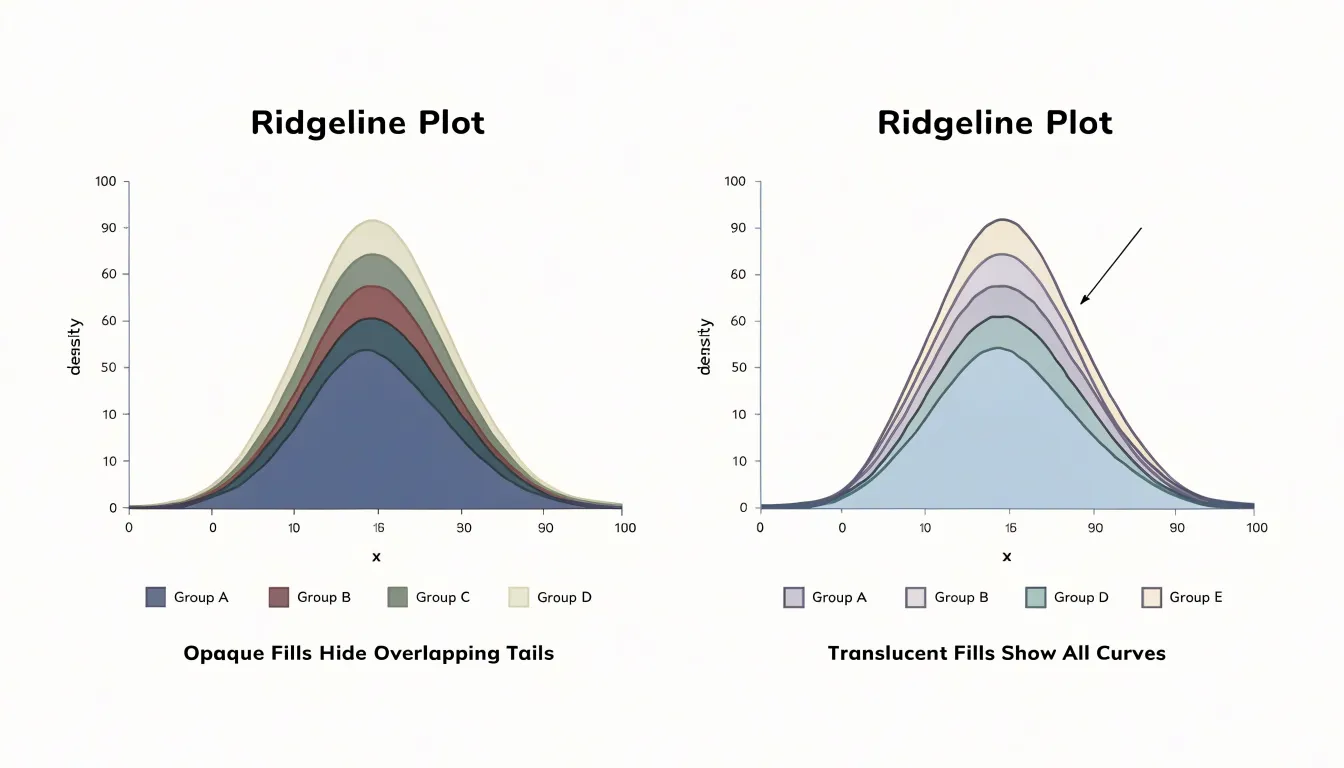
Overlap is the defining hazard of a ridgeline plot, and a handful of recurring design mistakes let it hide the very patterns the chart is meant to reveal. Excessive fill opacity tops the list. When each ridge is painted at or near full opacity, every curve covers the one behind it, so the tails of lower distributions vanish and only their peaks peek through. Keeping fills translucent, often in the range of half opacity or lighter, lets underlying shapes remain faintly visible and preserves the layered reading the chart depends on. Color choices compound the problem. Assigning similar hues to adjacent ridges blurs the boundary between them, while highly saturated or clashing palettes draw the eye to irrelevant variation and make overlapping regions read as visual noise. A restrained palette with adequate separation between neighbors keeps each distribution legible without turning the overlap into a single muddy mass. Bandwidth selection is equally consequential and often overlooked. Too small a bandwidth produces spiky, jagged ridges full of sampling artifacts that look like real structure, while too large a bandwidth smooths away genuine bimodality and subtle shoulders. Both extremes mislead: one invents detail, the other erases it. Because overlap hides data most stubbornly where distributions share the same values, these mistakes tend to cluster at the exact points an analyst cares about, masking trimodal shapes, long tails, and small secondary bumps. Reviewing a draft plot at full size, checking whether each curve’s outline stays traceable through its neighbors, and zooming into crowded regions all help catch these errors before they reach an audience. Small corrections to opacity, palette, and smoothing bandwidth restore the transparency of the display.
Axis Labels and Scales
Axis labels and scales carry much of the interpretive weight in a ridgeline plot, because viewers scan many stacked curves at once and rely on shared reference points to compare them. Configure tick marks so they appear at regular, intuitive intervals rather than at arbitrary positions generated by default plotting routines. A reader should be able to glance at any ridge and locate the corresponding value without counting gridlines or estimating fractions of a gap. Where the data spans orders of magnitude, choose the scale deliberately and label it explicitly.
A uniform horizontal scale across all ridges is essential. When each distribution occupies its own axis range, small values on one row and large values on another become visually indistinguishable, and the comparison the chart promises collapses. Fix the x-axis limits once, across the full figure, so that the position of a peak genuinely reflects its magnitude relative to every other row. Vertical placement identifies the category; horizontal position must remain constant in meaning.
Unit annotations belong close to the axis, stated plainly and consistently. Write ‘Temperature (°C)’ once with the shared axis rather than repeating a unit in every row label, and keep the same unit convention throughout. If the underlying data were transformed, note the transformation in the axis title so readers can convert values mentally. Place the axis label where it won’t collide with row names, often centered beneath the plot or aligned along the top.
Finally, tune typography for speed: legible tick label sizes, restrained gridlines that guide the eye without competing with the density curves, and consistent decimal precision. These details add up to an axis that recedes into the background while quietly making every value easy to read.
Software Options
Ridgeline charts have become a staple of modern exploratory data analysis, and a healthy ecosystem of software tools now supports their construction. In the R world, the ggridges package (formerly known as ggjoy) remains the reference implementation. Built directly on top of ggplot2’s grammar of graphics, ggridges supplies a geom_density_ridges() layer that handles the overlapping, vertically offset density curves that define the chart type. Users can control overlap, scale, and quantile line placement through simple parameters, and because it inherits ggplot2’s faceting and theming system, producing polished multi-group displays requires only modest code.
Python users typically turn to Seaborn, which offers a dedicated ridgeline-style function within its distribution plotting family. The function accepts long-format data frames and a grouping variable, drawing one density curve per category with configurable vertical spacing and translucent fills. Because Seaborn integrates with pandas and matplotlib, the resulting charts can be further customized or exported through the standard Python visualization stack, making it convenient for analysts already working in notebook environments.
Beyond these two dedicated libraries, general-purpose platforms round out the picture. Plotly provides ridgeline-like layouts through its subplot machinery in both Python and JavaScript, adding interactivity such as hover tooltips that static libraries lack. Business intelligence tools including Tableau and Power BI can approximate ridgelines using small multiples or layered density plots, though these require more manual configuration. Dedicated statistical environments like Stata and SAS offer community-contributed or built-in routines for the same purpose. Across all these options, the practical choice usually depends on the analyst’s existing workflow, the desired level of stylistic control, and whether the final output needs to be static, interactive, or embedded in a dashboard.
Real-World Examples
Ridgeline plots earn their place in real analytical work because they make change over many groups legible at a single glance. In meteorology, analysts use them to display temperature distributions month by month across a year or across several decades, stacking one density curve per month so that the seasonal shift appears as a flowing sequence of peaks. A climatologist can see at once how the cold tail of January compares with the warm center of July, and how those shapes have drifted over time. Demographic research offers another natural fit. Plotting age distributions for successive census years produces a ridge for each year, revealing the movement of population bulges, the thinning of younger cohorts, and the slow reshaping of a country’s age structure as it moves up the stack. The famous baby boom appears as a wave that travels diagonally through the chart rather than being buried in a table of numbers. Salary distributions benefit from the same treatment. When an organization plots income density by department, job level, or year, overlapping ridges expose where pay bands cluster, where long upper tails stretch toward executive compensation, and whether particular teams show unusual spread. Human resources analysts can compare the shape of one grade against the next and spot anomalies that averages would conceal. Performance tracking rounds out the picture. Teams monitoring response times, test scores, or delivery durations across quarters can plot a ridge per period, making improvements visible as shifts in the mass of the distribution rather than as a single moving average. Deterioration in the slow tail often shows up in a ridgeline before it registers anywhere else. Across all four domains, the common thread is the ability to compare many distributions without crowding the page, giving readers a compact visual narrative of how a population, a market, or a process evolves.
Dashboard Overview
A ridgeline plot earns its place in a dashboard when it is treated as one voice in a larger conversation rather than a standalone exhibit. The dashboard overview frames the plot within a hierarchy of information, placing summary metric cards along the top edge where they answer the immediate question of current state: totals, averages, and deltas that orient the viewer before any distribution is examined. Below this band, the ridgeline occupies a generous horizontal panel, typically spanning the full width or a two-thirds share, because its stacked densities need room to breathe and label cleanly. Secondary charts, such as time series for trend context or small bar charts for category comparisons, sit in narrower columns beside or beneath the ridgeline, reinforcing the story without competing for attention. Consistent color mapping across all panels ties the views together, so a category highlighted in a metric card carries the same hue in the ridgeline and in any supporting chart. Interactive elements deepen the connection: hovering over a ridgeline row can highlight the corresponding metric card, and clicking a card can filter the ridgeline to a single group. Axis alignment matters as well; sharing a common x-scale between the ridgeline and a companion histogram or trend line lets viewers read across panels without mental rescaling. Responsive layout rules keep the ridgeline readable on smaller screens by collapsing secondary charts into tabs while preserving the plot’s row spacing. Finally, a restrained set of annotations, such as a reference line marking a target or median, anchors the ridgeline to the dashboard’s broader narrative and prevents the visualization from feeling decorative.
Frequently Asked Questions
What is a ridgeline plot used for?
A ridgeline plot arranges many density curves or histograms in a vertical stack, with each row representing a distinct group, category, or time period. It lets you compare distributions across many groups using a shared horizontal axis for the quantitative variable.
How do you read a ridgeline plot?
Start by locating the group labels and confirming the order of the stack, then trace each row’s curve from its baseline upward to see where its mass concentrates. Comparing peak positions across rows shows shifts in typical values, while curve widths and tail lengths show changes in spread or secondary clusters.
What does a bimodal shape in a ridgeline plot mean?
A curve with two distinct humps and a dip between them is bimodal, which hints that two underlying populations or processes have been pooled together. Positive skew appears as a single long tail toward higher values, while negative skew piles observations at the high end and trails a thin tail toward lower values.
How much overlap should a ridgeline plot have?
A practical starting point is an overlap of roughly one half to two thirds of the row height, adjusted once the actual shapes are visible. Larger offsets with reduced overlap give each distribution more breathing room but make a taller chart.
Why does a ridgeline plot need a uniform horizontal scale?
A uniform horizontal scale across all ridges is essential so that the position of a peak genuinely reflects its magnitude relative to every other row. If each distribution uses its own axis range, comparisons across rows collapse.
What software can be used to make ridgeline plots?
In R, the ggridges package built on ggplot2 supplies a geom_density_ridges() layer for ridgeline plots. Python users typically turn to Seaborn, while Plotly, Tableau, Power BI, Stata, and SAS can also provide ridgeline-like layouts or routines.
Tony Astor
Tony writes about data visualization and the tools people use to build charts and dashboards. More about Data Illustrator