Polar Area Chart vs Pie Chart: Key Differences
 By Tony Astor ·

Polar Area Chart vs Pie Chart
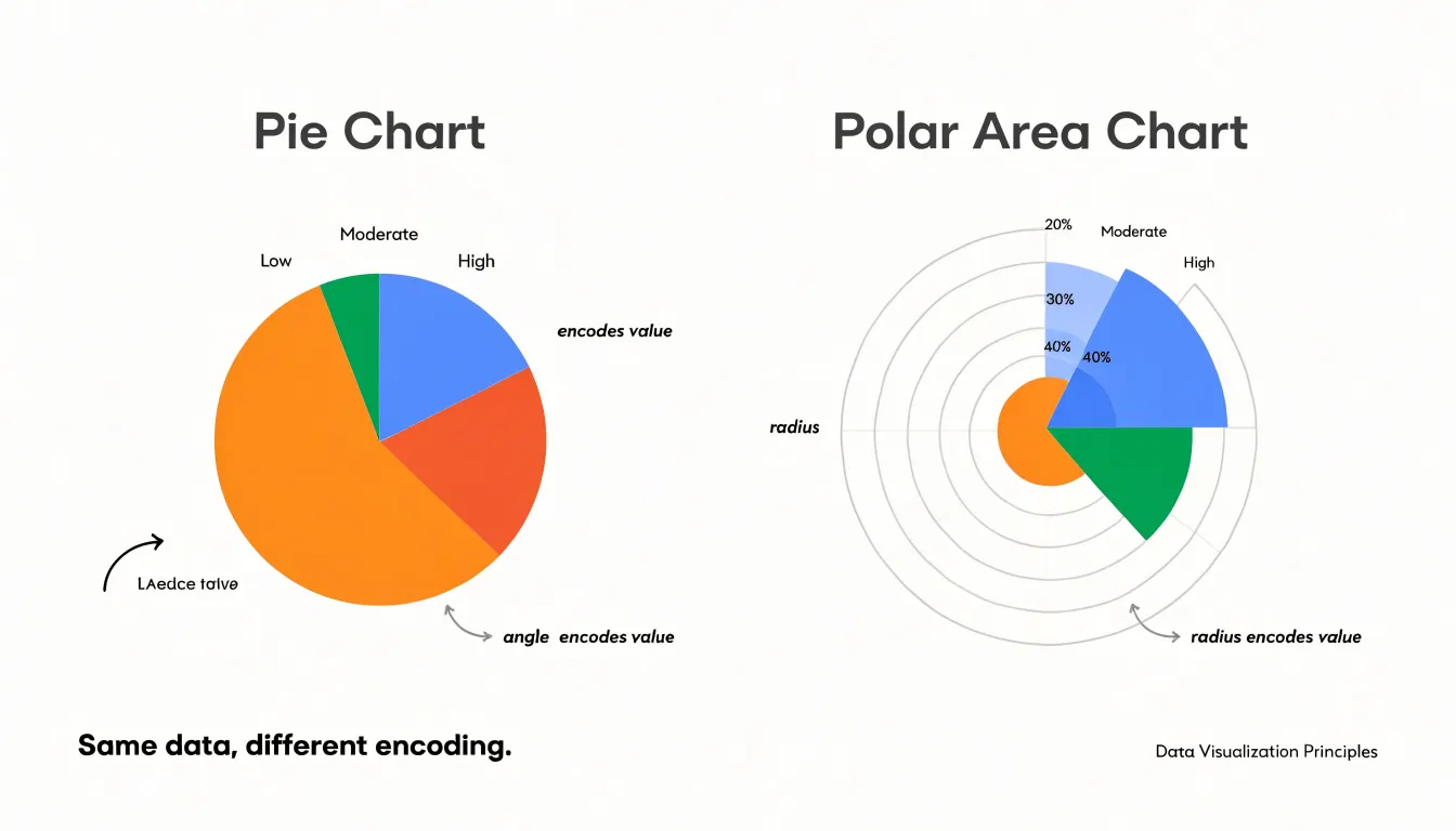
A pie chart shows parts of a whole as slices, with each slice’s angle proportional to its share, suiting small static datasets of five to seven categories. A polar area chart gives every category an equal angle but varies radius by value, better for cyclic data, many categories, and similar values.
Table of Contents
Pie Chart
A pie chart represents a single dataset as a circle divided into slices, where each slice corresponds to one category and the entire circle stands for the total. All slices sum to 100 percent, so the graphic communicates composition rather than change over time. Each category’s share is encoded as an arc, with the arc angle calculated by multiplying the category’s proportion by 360 degrees. A category holding a quarter of the total occupies a 90-degree arc, while a 10 percent share receives a 36-degree slice. This direct mapping between numerical proportion and geometric angle makes it easy to see which segments dominate and which are minor.
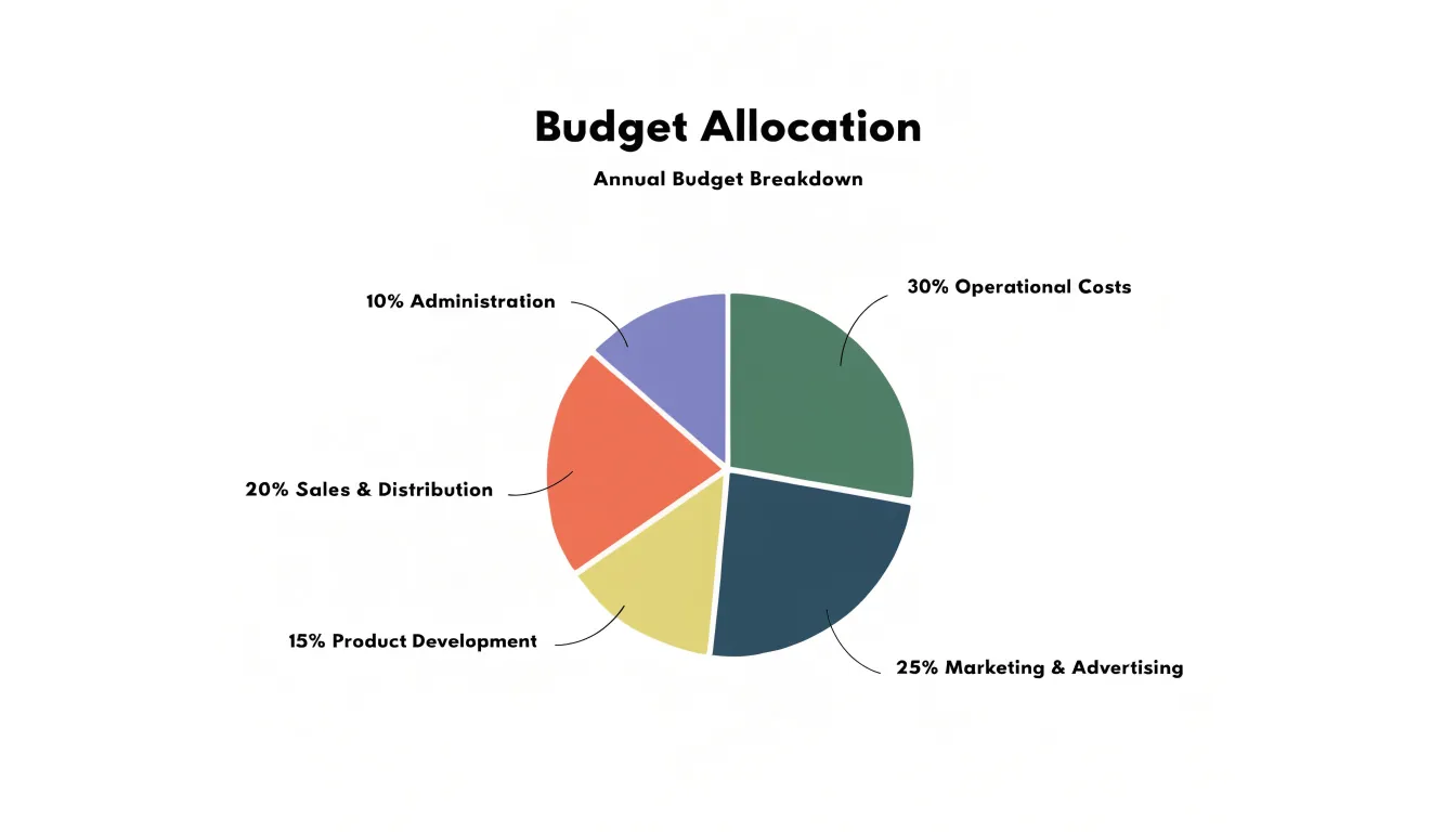
Pie charts work best for static data—a snapshot of a single moment or fixed period rather than a series of observations. The categories must be mutually exclusive and collectively exhaustive, so every unit in the population belongs to exactly one slice and nothing is left outside the circle. This structure suits questions like how a budget was allocated across departments in a given year, how a market splits among competing brands, or how survey respondents distributed themselves across answer options.
The chart type favors a small number of categories. With three to six slices, readers can compare arc sizes with reasonable accuracy and label each segment clearly. Because the chart depicts a fixed composition, it carries no inherent sense of sequence, hierarchy, or movement. The arrangement of slices around the circle is arbitrary, and the reader’s attention lands on relative area and angle rather than position. At a glance, the viewer perceives that the parts add up to a complete total and can identify the largest and smallest contributors without consulting a table.
Polar Area Chart
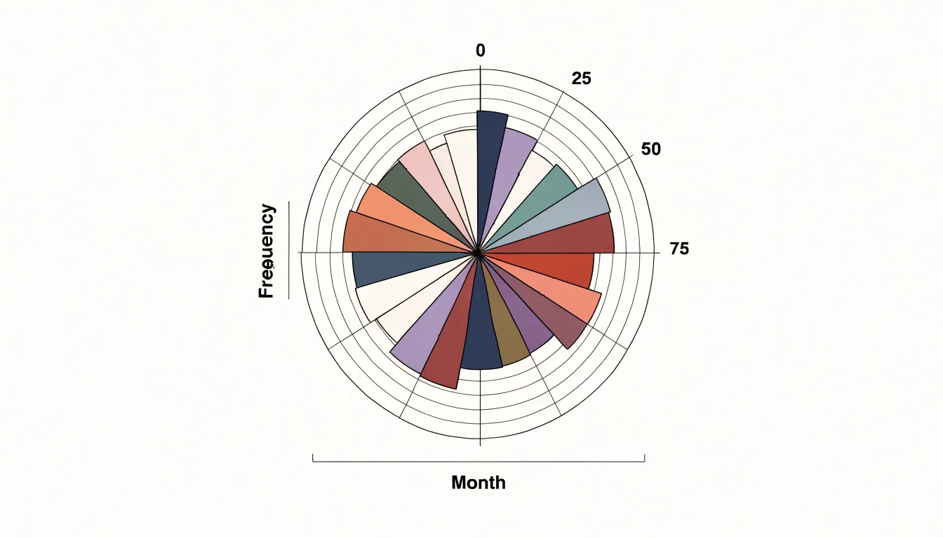
A polar area chart displays each category as a sector sweeping out from the center of a circle, with every sector assigned an identical central angle. Because the angular width is held constant, the sectors divide the circle evenly regardless of the underlying data. What varies is the radius: each sector extends outward to a length determined by its data value. A larger value produces a longer radius and a larger overall area, while a smaller value pulls the sector inward toward the center. This separates two visual properties that pie charts bind together, giving each category the same angular footprint while letting the radial dimension carry the quantitative message.
The Coxcomb chart, popularized by Florence Nightingale in her work on mortality statistics during the Crimean War, is the classic form of this design. The resulting diagram resembles a flower or a rose, with petals of different lengths radiating from a common center. Because every sector occupies the same angle, viewers can compare categories by looking at how far each sector reaches outward from the center point. The equal-angle foundation also keeps the overall shape balanced, allowing the chart to function as a compact circular display for datasets with many categories or a cyclical structure.
Visual Mechanics
While both chart types use angular sweeps around a shared center, they rely on different secondary visual channels. In a pie chart, every slice shares the same radius, so all variation is carried by the angle and the arc length at the rim. In a polar area chart, each segment keeps a constant angular width, and the value is expressed by radial extension, meaning the segment’s area grows with the square of that radius. This difference matters because the human visual system does not treat angular extent and area as interchangeable currencies of comparison.
Perceptual research shows that people estimate lengths and positions along a common scale with reasonable accuracy, while judgments of area and volume tend to be systematically compressed. When two pie slices sit side by side, a reader can compare the arcs at the outer edge, and the eye is fairly good at registering that one sweep covers more of the circle than another, especially when the difference is modest. The common baseline of the shared radius gives every slice the same starting reference, reducing the comparison to a simple angular judgment.
In a polar area chart, the comparison becomes an area judgment between wedges whose outer boundaries curve at different distances from the center. Because area scales quadratically with radius, viewers routinely underestimate this growth, and the lack of a shared outer boundary removes the reference line that makes pie slices easy to line up against one another. Consequently, polar area charts demand more careful reading of the radial extent, often with gridlines or labeled ticks, while pie charts lean on arc length for quick relative judgments.
Cyclic Time Data
Cyclic time data—such as months of the year, hours of the day, or days of the week—possesses an inherent circular structure that linear representations often fail to capture. A polar area chart accommodates this by mapping time periods around a full 360-degree circle. Each period receives an equal angular slice, and the radial length encodes the value. Viewers can perceive the seamless progression from one cycle to the next, as the end of the circle connects directly back to the beginning.
When pie charts are used for cyclic data, they impose an artificial start and stop boundary. Representing 12 months as pie slices forces a linear reading from January to December, with a distinct break between the end and the beginning that disrupts continuity and can obscure repeating seasonal patterns. By using radius to encode magnitude, the polar area chart avoids the need to sum parts to a whole and instead emphasizes the rhythmic rise and fall of values across the cycle.
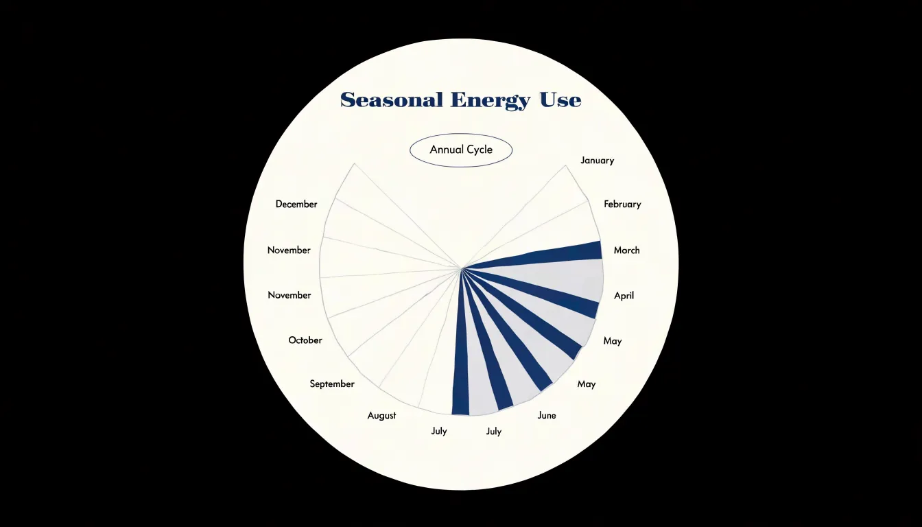
Seasonal patterns, such as peak energy consumption in summer or low website traffic on weekends, become immediately apparent as radial lengths wax and wane around the circle. The continuous circular layout also helps identify phase shifts and trends over multiple cycles when data for several years are overlaid or displayed in concentric rings.
Similar Data Values
When data values are similar, the choice of chart type can determine whether those differences are perceptible at all. In a pie chart, if two categories have values of 48 and 52, their angles are 172.8 and 187.2 degrees—a difference of just 14.4 degrees. On a chart a few inches across, that translates to a sliver so thin that most viewers will see the slices as effectively equal. The visual system is not well tuned to compare close angles, especially when slices are separated by other categories, compressing meaningful variation into a nearly uniform ring.
A polar area chart handles the same values through radial length, which is easier to discriminate than angle when starting from a common center. A value of 48 versus 52 produces radii that differ by about 8 percent. On a chart with a two-inch radius, that is a visible gap of roughly 0.16 inches at the outer edge, which the eye can detect with reasonable reliability. Furthermore, because segment area scales with the square of the radius, the visual weight of the larger value is amplified, making subtle variations among similar values stand out clearly.
Large Datasets
Pie charts carry a practical ceiling once the number of categories climbs beyond roughly five to seven slices. Small wedges become difficult to distinguish, adjacent colors compete at thin boundaries, and labels must shrink, rotate, or migrate to a legend where the connection between name and slice is lost. As more categories are added, the smallest slices compress into slivers that are nearly impossible to compare, forcing readers to scan a legend repeatedly rather than reading the data directly.
Polar area layouts handle higher category counts with more composure. Because each category occupies a fixed angular sector, segments remain anchored in place regardless of how small their values become. Adding categories simply divides the circle into more evenly spaced sectors, allowing dozens of categories to coexist without crowding.
Radial length also gives small values more room to register. A modest value near the center of a polar area chart still produces a visible spoke with a defined edge, whereas the equivalent proportion in a pie chart collapses into a hairline wedge. Labels can be placed around the perimeter at regular intervals, keeping each category name adjacent to its segment.
Visual Misconceptions
When a polar area chart maps values directly to the radius of each segment, the visual impression does not follow the data in a straight line. Viewers judge the size of each wedge by the amount of colored area it occupies, which grows with the square of the radius. Doubling a value and doubling the radius produces a wedge with four times the visible area, exaggerating the differences between segments.
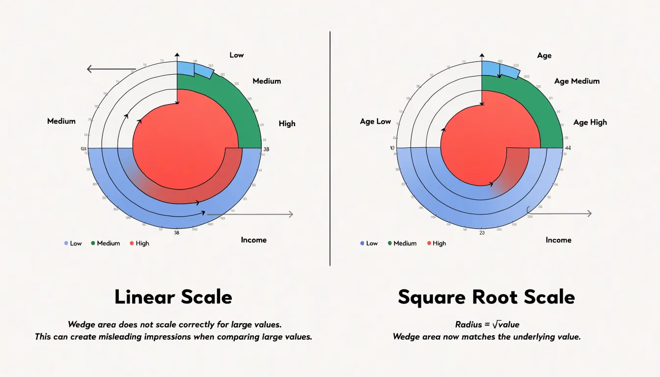
This effect matters most at the larger end of the scale. Segments with small radii stay compact even when their underlying values differ meaningfully. Segments with larger radii expand quickly, and each increment in value adds a disproportionate band of color around the outer edge. Viewers tend to anchor their reading on those dominant wedges, overestimating the values they represent and underestimating the smaller ones by comparison.
The standard fix is to scale the radius by the square root of the value rather than the value itself. Because area is proportional to the square of the radius, applying the square root makes the resulting area proportional to the underlying value. A segment representing four times as much as another then covers four times the area, matching how viewers intuitively read the chart.
Best Uses for Pie Charts
Pie charts excel when the audience needs to grasp relative proportions at a glance:
- Binary survey results: When a poll asks whether respondents support or oppose a proposal, a two-slice pie chart communicates the split instantly, showing which side holds the majority and by how wide a margin.
- Market share splits: When a handful of competitors divide a market, a pie chart shows the hierarchy of dominance without requiring readers to consult axis labels or scales, making it effective in executive summaries, presentations, and infographics where space is limited.
- Household budgeting: Allocating monthly income across housing, food, transport, utilities, and savings reflects a complete whole divided into parts. Slices that grow or shrink from month to month signal where spending pressure is building.
Pie charts serve these goals best when proportions differ noticeably, precise comparisons between similar slice sizes are unnecessary, and accompanying text supplies the exact figures.
Ideal Cases for Polar Area Charts
Polar area charts shine when a dataset combines magnitude with direction or cyclic time, where the angular position around the circle carries meaning:
- Wind rose meteorology: Each compass sector holds the frequency of wind arriving from that bearing, with segment length showing how often the wind blew from each direction. The layout mirrors the physical compass, giving meteorologists an immediate profile of prevailing winds and seasonal shifts.
- Seasonal crime statistics: Placing January through December around the circumference lets each month’s segment length express incident volume. Readers can spot summer spikes or holiday-period increases and compare one year’s ring against another’s at a glance.
- Cyclic performance metrics: Website traffic by hour of day, call-center volume by day of week, production output by shift rotation, and energy consumption across the four seasons all involve recurring intervals. A polar area chart keeps that cyclical context visible, whereas a bar chart presents a linear sequence that hides the return to the starting point.
Color and Contrast
Effective palette selection begins with visual separation: adjacent sectors must differ enough in hue, lightness, or saturation for the eye to trace each boundary without effort. A common method is to choose a base hue and step its lightness systematically so neighboring slices differ by a clear increment while retaining a family resemblance. Alternatively, an evenly spaced hue wheel can select colors at regular angular intervals so no two adjacent slices share a similar tone. In both approaches, testing the palette in grayscale is a quick check, since sectors that merge into the same gray value will also blur together for viewers with color vision deficiencies.
Restraint is equally important. Too many saturated colors create visual fatigue, and the eye loses track of which color belongs to which sector. Limiting a palette to a modest set of tones—reserving the brightest or most saturated color for the sector that deserves emphasis and using muted or desaturated tones for the rest—keeps attention focused. A legend placed close to the chart with exact color swatches further reduces cognitive load.
Finally, background context matters. A dark background calls for lighter, higher-contrast tones, while a light background benefits from deeper shades. Consistent use of the same palette across related charts helps readers carry color associations from one figure to the next.
Accessibility
A meaningful share of any audience perceives color differently from the designer, including those with common red-green or rarer blue-yellow color vision deficiencies. When a chart relies on color alone to distinguish segments, these viewers can lose the boundaries between slices entirely.
To make circular charts accessible, never let a single visual attribute carry information on its own:
- High-contrast borders: A thin stroke in a dark neutral tone, or in white against darker fills, separates adjacent segments even when their hues appear nearly identical to a colorblind viewer.
- Patterns: Diagonal lines, dots, crosshatching, and solid fills can be combined so every segment differs from its neighbors in texture as well as color. A viewer who cannot separate red from green can still separate stripes from dots.
- Direct labeling: Attaching category names and values inside or immediately beside each segment removes the need to match a slice to a distant legend—a task that becomes impossible when several legend swatches look alike.
Common Design Mistakes
Polar area charts and pie charts are especially vulnerable to design practices that quietly distort what readers perceive:
- Three-dimensional effects: Rendering a chart with depth makes foreground slices or wedges appear larger than slices of identical value placed toward the rear, meaning area and angle no longer correspond reliably to the numbers.
- Exploded slices: Pulling one segment away from the rest draws disproportionate visual attention to a category that may not deserve emphasis and breaks the overall shape readers use to judge proportions.
- Non-zero radial baselines: In a polar area chart, if the radius scale starts above zero, spoke length no longer maps proportionally to its value, exaggerating small differences between categories. Starting the scale at zero keeps the encoding truthful.
- Missing labels: Unlabelled segments force readers to guess at categories and values. Every segment requires a readable direct label or an unambiguous key.
Quick Decision Framework
Before committing to either chart type, run through three diagnostic questions in order:
- Dataset size: How many categories must the chart display? Choose a pie chart for five to seven slices or fewer; switch to a polar area chart when categories multiply and angles would shrink too much to distinguish.
- Cyclic nature: Do the categories represent parts of a single whole or recurring periods across a cycle? Use a pie chart for discrete compositional breakdowns (market share, budgets) and a polar area chart for continuous rings of time or direction (months, seasons, hours).
- Analytical depth: Must viewers compare individual values precisely or simply grasp overall proportions at a glance? A general audience needing the broad shape of a distribution is well served by a pie chart, while analysts comparing magnitudes across many categories benefit from the radial encoding of a polar area chart.
Final Comparison Checklist
To turn the preceding analysis into a repeatable decision tool, evaluate your dataset against two groups of criteria:
- Data features: Compare how each chart handles the number of categories, similarity in magnitude between values, cyclical or directional patterns, the number of series displayed, and the need for precise value reading versus a general impression of proportion.
- Visual performance metrics: Assess accuracy of proportion estimation, discriminability between adjacent segments, sensitivity to small value differences, scalability as categories are added or removed, and visual stability when underlying data updates.
When the data consists of a small set of parts that sum to a whole and the audience only needs an approximate sense of proportion, use a pie chart. When the data is cyclical, directional, larger in category count, or requires comparing similar values with precision, use a polar area chart.
Frequently Asked Questions
What are pie charts best used for?
Pie charts are best for a single dataset shown as parts of a whole, especially static data with mutually exclusive categories and a small number of slices. They work well with three to six slices, and the article notes a practical ceiling beyond roughly five to seven slices.
What is the difference between a polar area chart and a pie chart?
A pie chart keeps every slice at the same radius and varies the angle, while a polar area chart keeps each sector’s angle constant and varies the radius to encode value. Because a polar area chart’s segment area grows with the square of the radius, it often needs careful reading with gridlines or labeled ticks.
Can a polar area chart show months of the year or hours of the day?
Yes, a polar area chart can map cyclic time data such as months, hours, or days around a 360-degree circle, with equal angular slices and radial length encoding the value. The article notes that pie charts impose an artificial start and stop boundary that can disrupt continuity for cyclic data.
Which chart is better for showing very similar values?
A polar area chart can make similar values easier to discriminate because radial length differences are easier to compare than close angles in a pie chart. However, the article notes that because area scales with the square of the radius, the radius should be scaled by the square root of the value to keep area proportional.
Can a pie chart handle a large number of categories?
Pie charts have a practical ceiling once categories climb beyond roughly five to seven slices, because small wedges become difficult to distinguish and labels may shrink, rotate, or move to a legend. Polar area layouts handle higher category counts better because each category keeps a fixed angular sector.
How can I make circular charts accessible for colorblind viewers?
The article recommends never letting color alone carry information: use high-contrast borders, patterns, and direct labeling so segments can be distinguished by other visual cues. It also suggests testing the palette in grayscale to check whether neighboring sectors blur together.
Tony Astor
Tony writes about data visualization and the tools people use to build charts and dashboards. More about Data Illustrator