Polar Area Chart: How It Works and How to Read It
 By Tony Astor ·
Polar Area Chart
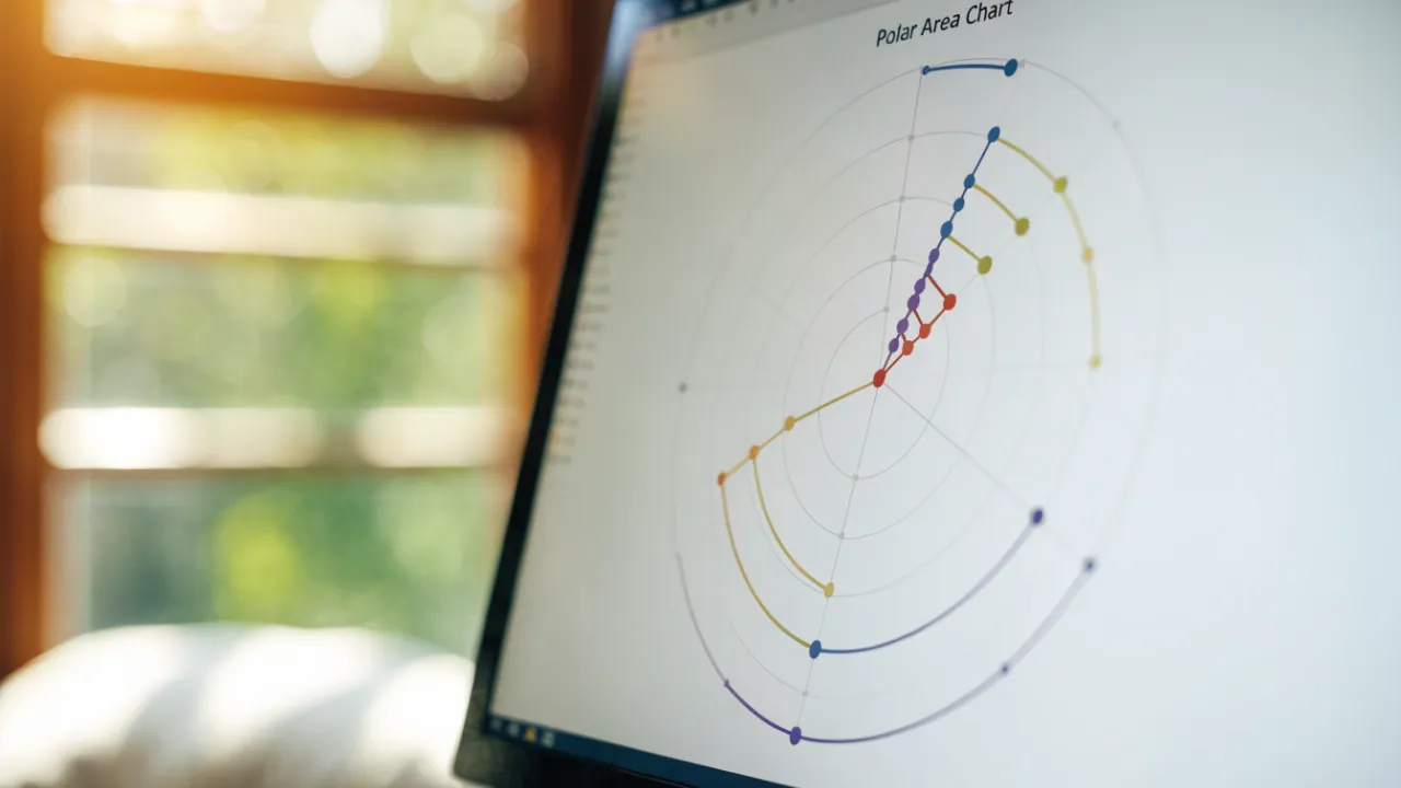
A polar area chart is a circular statistical graphic where categories are arranged as equal-angled sectors around a common center, with each category’s value encoded by its sector’s radius rather than its angle. Popularized by Florence Nightingale in the 1850s as the Coxcomb or rose chart, it suits cyclical data but can distort perceived magnitude.
Table of Contents
- Polar Area Chart
- Pie Charts vs Polar Charts
- Slice Radius and Angles
- Historical Origins
- Reading the Chart
- Continuous Time Visuals
- Sorting Data
- Color Coding
- Common Reading Pitfalls
- Ideal Use Cases
- Poor Fit Scenarios
- Preparing Data and Choosing Software Tools
- Customizing Scales and Overlaying Multiple Datasets
- Real World Examples
- Design Best Practices and Interactive Dashboards
Polar Area Chart
A polar area chart, historically known as a Coxcomb chart or Nightingale rose chart, is a circular statistical graphic in which data categories are arranged around a common center as equal-angled sectors, with the value of each category encoded by the radius of its sector. Popularized by Florence Nightingale in the 1850s, the chart takes the name “Coxcomb” from the rosette-like appearance of the resulting figure.
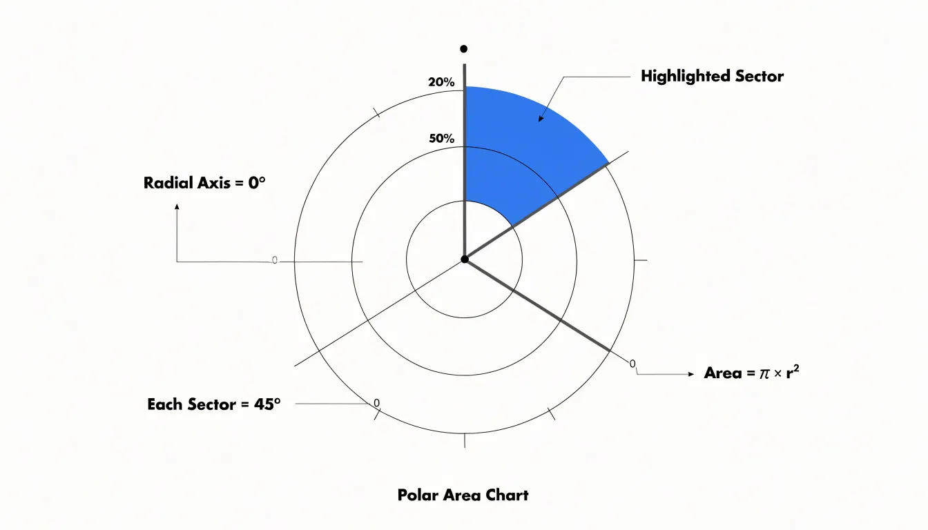
The structural anatomy of the chart follows a consistent geometry. The full 360 degrees of the circle is partitioned evenly among categories: a chart with eight categories gives every sector a central angle of 45 degrees; with ten categories, 36 degrees; with five, 72 degrees. Each sector begins at the center point, extends outward along two bounding radii, and terminates at an outer arc whose distance from the center varies from sector to sector. Because the angular extent remains fixed, the radial extent serves as the encoding channel.
A category with twice the value of another receives a radius twice as long, producing a visibly larger sector. Because both the radius and the arc length grow with the value, the enclosed area of each sector scales with the square of the radius. Careful labeling of radial intervals, or the inclusion of concentric reference rings, helps viewers estimate values accurately across the full range of plotted data.
Pie Charts vs Polar Charts
A pie chart and a polar area chart both place data around a circle, yet they encode magnitude in different geometric dimensions. In a pie chart, every slice shares the same radius, and the value is expressed through the central angle: a category worth twice as much occupies twice the sweep of arc. The circle’s overall size stays fixed, so the eye reads proportion by comparing wedge widths at the rim. A polar area chart holds the angles constant instead and lets the radius of each sector grow or shrink with its value.
This difference in geometry shapes how readers interpret the chart. Angle comparisons in a pie chart are relatively easy for the eye to judge, particularly for halves, quarters, and thirds, since the landmarks are familiar and the outer edge lines up neatly. When the encoding shifts to radius, perception changes: people tend to underestimate differences in area, and because a slice with double the radius covers four times the area, the chart can exaggerate or distort the impression of magnitude.
The equal angles of a polar chart do offer an orderly frame, giving each category a fixed position around the circle so readers can track a series of categories without the shifting boundaries that pie layouts produce. The trade-off is that the area of each wedge carries the visual weight, and area judgments are less precise than angle judgments. Readers comparing adjacent sectors may also find that the radial extent of one slice bleeds visually into its neighbor, especially when values are close.
Slice Radius and Angles
In a polar area chart, the area of each slice is proportional to the square of its radius multiplied by its fixed angular fraction. Because every slice starts from the same baseline geometry and shares a common vertex at the center, the consistent wedge angles make the outer arc lengths directly comparable across categories.
Where values are similar, the outer edges align into a nearly circular profile; where values diverge, the profile becomes jagged, with long spikes and short stubs. This fixed angular symmetry allows the radius—and therefore the value—to stand out against a uniform structural framework.
Historical Origins
Florence Nightingale devised what she called the “rose diagram” while serving as a nurse administrator during the Crimean War. Working from the Barrack Hospital at Scutari, Nightingale gathered detailed mortality statistics on British soldiers and became convinced that the vast majority of deaths came from disease and unsanitary conditions rather than battlefield wounds.
To communicate this finding to cabinet ministers, military officials, and Members of Parliament who would never read a statistical table, she developed a graphic in which each month of the year occupies an equal wedge around a circle, and the area of each wedge grows in proportion to the monthly death toll. The result was a wheel of unequal petals that made seasonal surges of preventable mortality immediately visible.
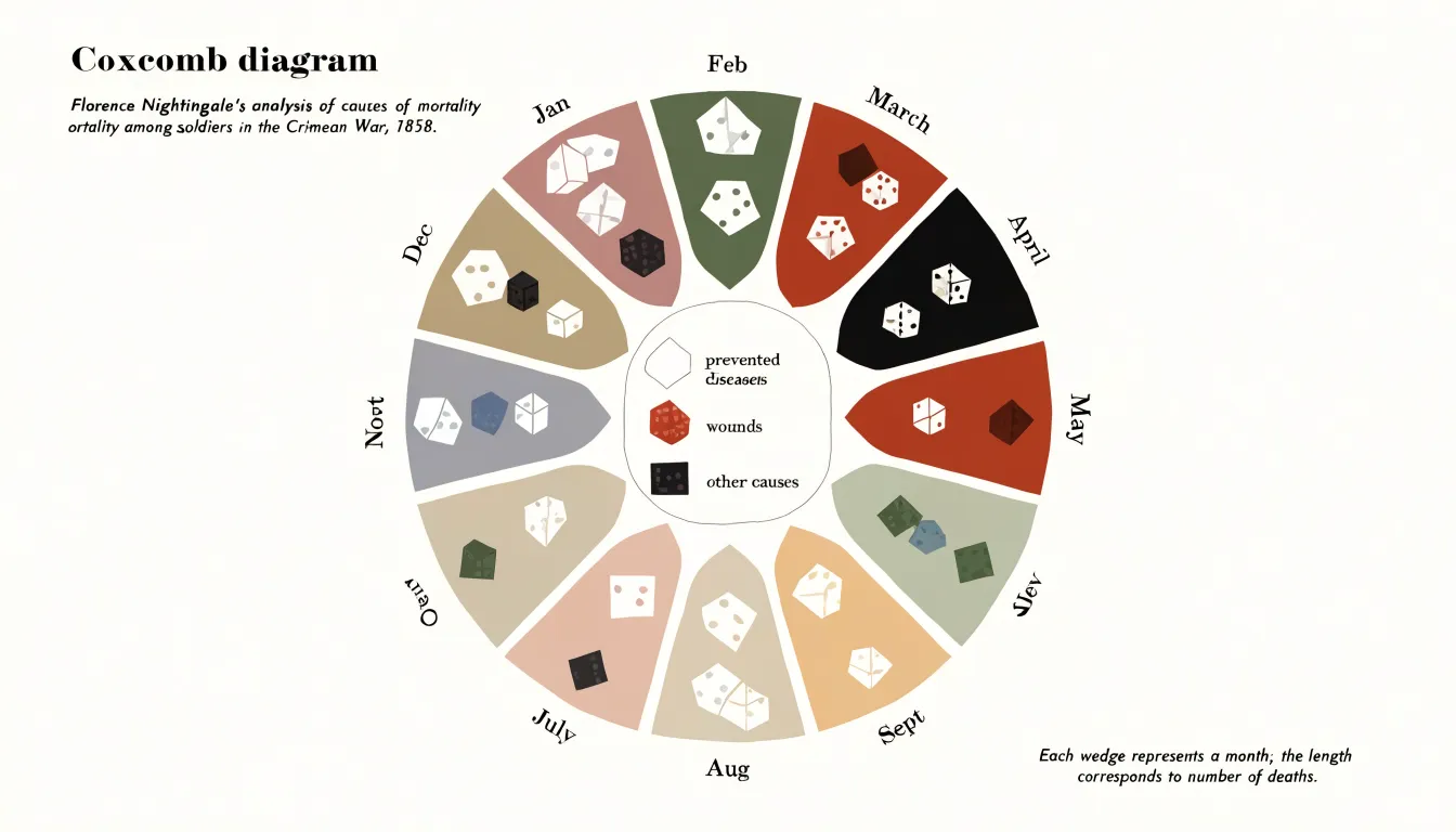
Nightingale financed the printing of her diagrams herself and circulated them widely among policymakers alongside explanatory pamphlets. The charts helped lead to the establishment of the Royal Commission on the Health of the Army and to sweeping reforms in military barracks, hospitals, and sanitation.
Reading the Chart
To read a polar area chart accurately, begin at the center point (zero), which serves as the origin for all quantitative values. Follow a segment outward and note where its outer edge intersects the radial scale—typically concentric circles or grid lines marked with numeric values. This intersection point gives the category’s quantitative value.
Next, verify that the boundaries between segments are evenly spaced around the circle. Equal angular spacing ensures that differences in segment size are due solely to variations in the quantitative value.
When comparing segments, focus on the radial extent rather than the visual area. Because area is not directly proportional to the value in a standard radius-encoded polar chart, always measure values by tracing the distance from the center to the outer edge against the concentric scale.
Continuous Time Visuals
Seasonal and periodic data carry an inherent circular rhythm that polar area charts are well suited to express. When rainfall is measured month by month, the data returns to its starting point after twelve steps, forming a loop rather than a line. A polar area chart maps each month to an angular slice around the compass, so January sits beside December just as it does on a calendar. Wet months extend outward while dry months remain close to the center, letting readers recognize the rainy season as a spike that recurs at the same angle each year. Comparing two years side by side becomes a matter of overlaying two rings and observing how the petals align or shift, revealing whether a monsoon arrived early, late, or with unusual intensity.
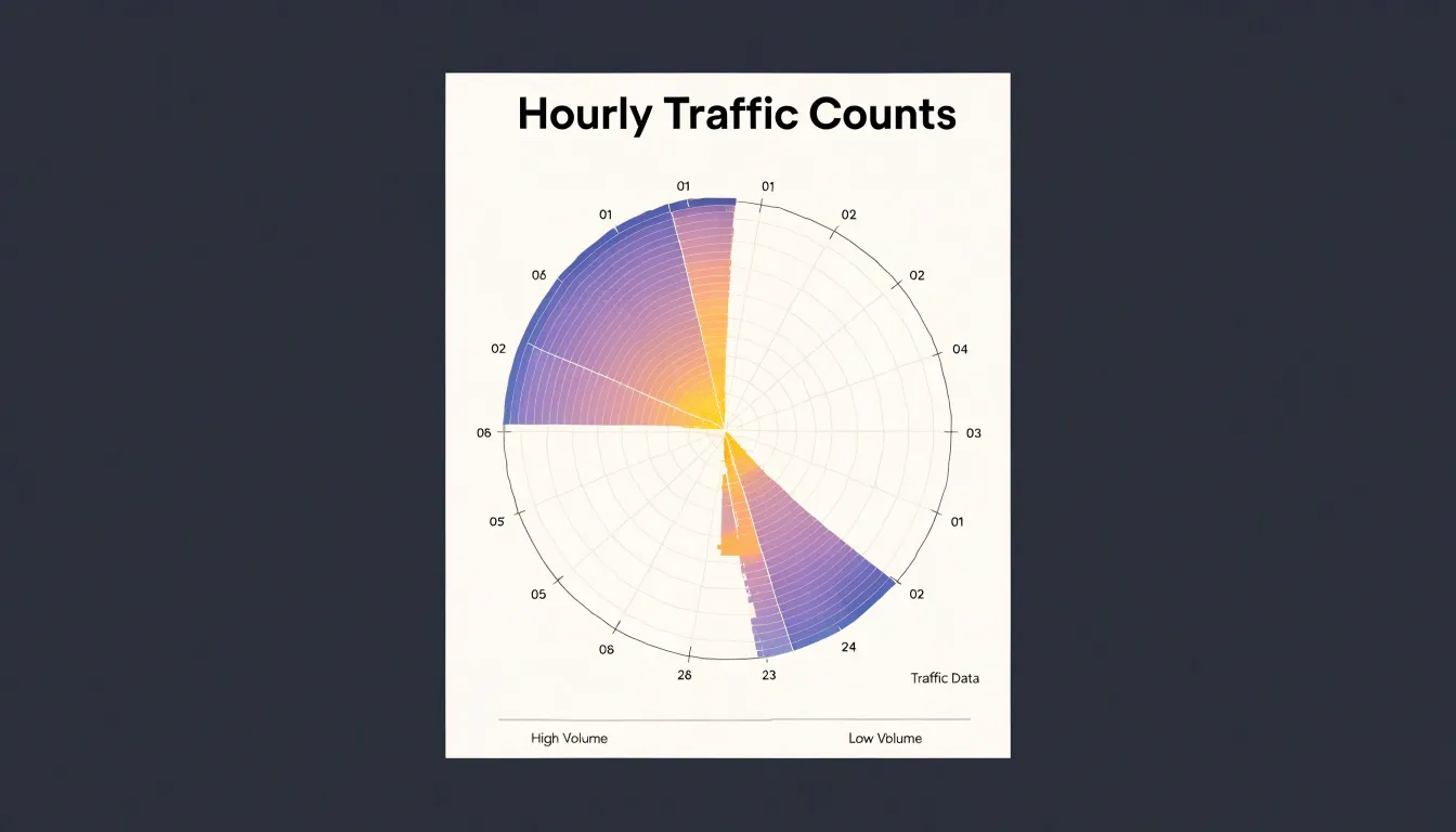
The same logic applies to hourly traffic counts. A polar chart with twenty-four angular slices turns the daily commute into a visible pair of bulges at the morning and evening rush, while weekend patterns appear as distinct indentations in the ring. Because the eye is sensitive to symmetry and repetition, cyclical irregularities stand out immediately: a flat ring signals steady conditions, while an asymmetric one points to an anomaly at a specific time of day or year. This makes the chart a useful diagnostic tool for monitoring recurring phenomena such as utility demand or customer footfall.
Sorting Data
The order in which sectors appear around a polar area chart influences how easily readers extract meaning. A magnitude-based ordering places the largest sectors together and progresses smoothly down to the smallest, creating a visual gradient that guides the eye around the circle and communicates hierarchy without forcing the reader to hunt across the chart. For time-based data, ordering sectors chronologically preserves the narrative flow so that seasonal shifts, growth trends, or recurring cycles emerge as continuous waves rather than scattered fragments.
Random or arbitrary ordering introduces friction. Sectors of wildly different sizes sit side by side, forcing the reader to jump back and forth to compare non-adjacent wedges. This visual clutter obscures trends and can suggest false relationships between neighboring sectors that sit next to one another by accident.
Color Coding
When sectors are adjacent, similar hues can blur together. Selecting colors with sufficient perceptual distance—through variation in hue, saturation, or lightness—ensures that each slice remains distinct so viewers can compare radial lengths without visual interference. Alternating light and dark tones or using a qualitative palette with clearly separated hues prevents confusion between neighbors.
When the goal is to highlight specific target metrics, such as a sector that exceeds a threshold or represents a key performance indicator, a contrasting accent color draws attention without requiring extra annotations. Restraint is essential: using too many bright or saturated colors overwhelms viewers, whereas a limited palette with a few highlighted colors keeps the chart focused. Maintaining consistent category colors across multiple charts also helps viewers build familiarity.
Common Reading Pitfalls
When a viewer looks at a polar area chart, the brain judges a wedge’s size by its total area rather than by its radius. Because area grows with the square of the radius, a segment with twice the radius covers four times the area, yet the visual system also compresses large ratios and inflates small ones. Wedges that differ modestly in radius can look more similar than they are, while wedges with large gaps in value look exaggeratedly different. As a result, rankings and proportions read by eye may not match the underlying numbers.
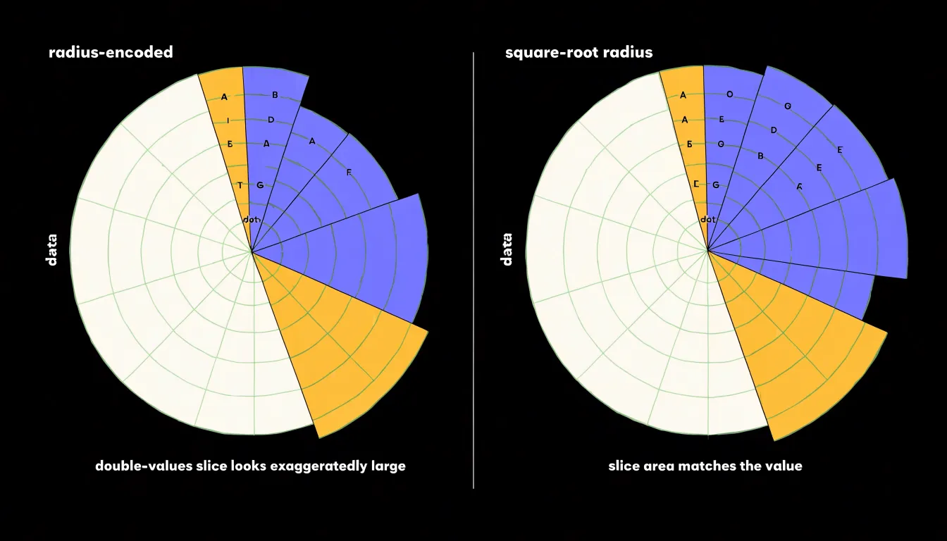
Several strategies reduce this bias:
- Add direct numeric labels on each segment so readers can verify values without relying on visual estimation.
- Map the encoded quantity to area rather than radius (using a square-root scale for the radius), aligning the visual impression with the data.
- Keep the number of segments small to avoid crowding and compounding estimation errors.
- Include clearly marked reference rings and consistent scaling across all segments as fixed anchors for judging size.
- Order segments by value and pair the chart with a companion bar chart so readers can use the polar view for pattern recognition and the linear view for exact figures.
Ideal Use Cases
Polar area charts excel where data has a natural radial, directional, or cyclical structure:
- Directional wind rose plotting: Wind speed or frequency recorded across compass directions maps naturally to sectors around a circle, allowing viewers to spot prevailing wind patterns and directional biases that would be cumbersome to interpret in a linear bar chart.
- Cyclical periodic metrics: Hourly energy consumption, daily website traffic, and seasonal sales figures benefit from mapping time periods onto angular sectors to highlight peaks and troughs relative to the cycle.
- High-level dashboard summaries: Because the radial layout accommodates multiple categories in a compact space, it works well on executive dashboards or monitoring screens where the goal is to convey overall status and spot outliers at a glance.
Poor Fit Scenarios
In many scenarios, standard linear bar charts prove more effective than polar area charts:
- Subtle value differences: The human eye is better at comparing lengths along a common baseline than judging differences in sector area or radius. When values differ by only a few percentage points, aligned bars make those differences apparent, whereas a polar chart obscures them.
- Non-cyclical datasets: Polar area charts imply a cyclical or directional relationship among categories. Arranging arbitrary categories around a circle can mislead viewers into perceiving patterns that do not exist, whereas a linear bar chart supports natural ranking without implying false cycles.
- Dense metrics: With many categories or fine-grained data points, labels crowd the perimeter of a polar chart and sectors shrink to unreadable slivers. Bar charts handle density by extending along a single axis with readable labels, consistent spacing, and gridlines for precise reading.
Preparing Data and Choosing Software Tools
Each slice of a polar area chart requires a category label and a corresponding positive numeric value. Organize the data into a simple two-column structure, with categories in one column and values in the adjacent column; for multiple series, place each series in its own column sharing the same categories. Because a radius cannot be meaningfully negative, values must be positive, and zero values will collapse to a single point at the center. Handle missing data deliberately by removing affected rows or substituting a neutral value so the remaining slices are not distorted.
Once the data is tidy, software options vary in how much control they offer:
- Excel: Lacks a native polar area chart type, so users commonly transform category values into angles and radii and plot the result on a scatter chart with smoothed lines and filled shapes.
- Tableau: Supports radial visualizations through calculated fields that convert category positions into angles and values into radii, an approach that scales well for interactive dashboards.
- R (ggplot2): Provides dedicated polar coordinate functionality (
coord_polar), letting analysts build custom polar area charts by combining bar geometries with polar coordinates and adjusting fill and transparency. - Python (Matplotlib): Offers a polar projection in the
pyplotmodule that supports bar-like drawing at specified angles, onto which analysts can layer styling, labels, and legends.
Customizing Scales and Overlaying Multiple Datasets
Selecting an appropriate maximum value on the radial axis prevents smaller segments from becoming indistinguishable. Setting a minimum baseline other than zero can amplify differences among values that cluster within a narrow range, though this compresses the visual area dedicated to each unit and may exaggerate minor variations. Any baseline adjustment must be applied uniformly across all segments.
When overlaying multiple datasets, the goal is to reveal relationships without letting the upper layer obscure background sectors:
- Use partial transparency on the secondary dataset, or place the comparative dataset behind the base sectors as a subtle backdrop.
- Apply distinct visual encodings for the overlay, such as an outlined radial line, a patterned fill, or a different stroke width.
- Slightly offset the overlay’s radius when multiple datasets share the same angular segments to separate the series visually.
- Test at multiple sizes to verify that overlays remain legible and scale adjustments do not introduce distortions.
Real World Examples
Meteorologists use polar area charts to compare climate profiles across weather stations. A monthly precipitation chart places twelve wedges around the circle with radial length representing average rainfall in millimeters. In a temperate climate, long spokes appear for late-winter and spring months and short spokes for dry summers; a coastal station with a pronounced wet season produces a lopsided wheel, while an inland station with evenly distributed rain yields a near-circular shape. Similarly, plotting mean monthly high temperatures reveals a smooth swell peaking around July in the northern hemisphere, making anomalies—such as an unusually warm October pushing its wedge outward—easy to spot.
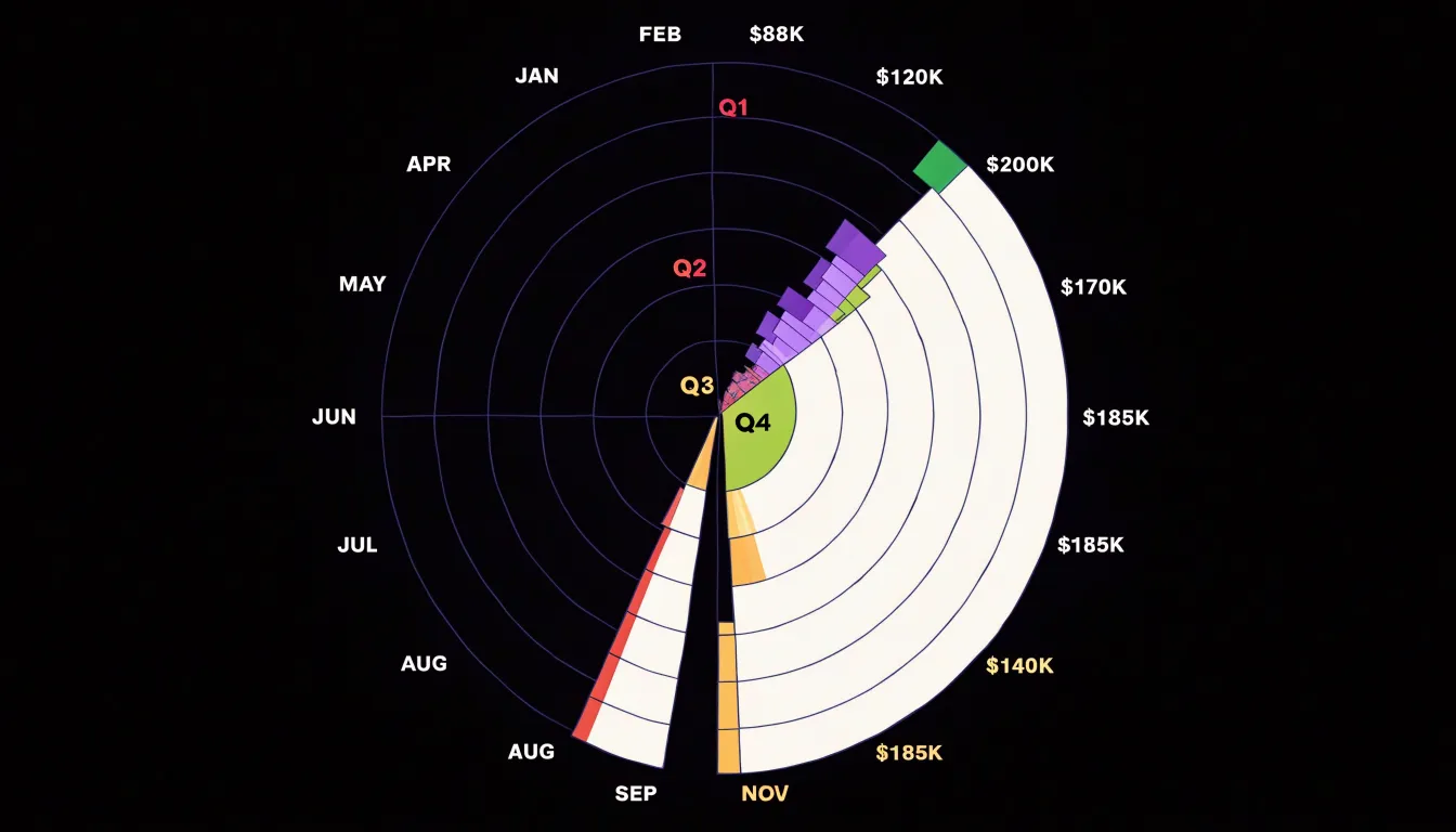
Retail revenue also maps well onto fiscal quarters. A retailer can divide the chart into four quarterly wedges, subdivided by month to preserve twelve-slice granularity. Holiday-driven businesses typically show dramatic elongation in the fourth quarter, compressing the remaining months into modest slivers. Comparing several years on the same chart, or juxtaposing charts for different store locations, exposes how consistently revenue concentrates in the final quarter and whether promotional efforts have flattened or sharpened that peak.
Design Best Practices and Interactive Dashboards
When deploying a polar area chart in an interactive web dashboard, surround the graphic with clear labeling and responsive controls:
- Tooltips: Configure each slice to respond to hover (and touch on mobile devices) with a compact panel showing the category name, exact value, and share of the total. Position tooltips so they never cover the inspected slice.
- Dynamic legends: Allow users to toggle categories on and off—especially helpful when many slices crowd the outer ring—and update legend styling to reflect hidden items. On narrow screens, legends should collapse gracefully.
- Hover states: Use a subtle highlight or slight outward offset on the active slice to reinforce the connection between legend, tooltip, and chart, keeping transitions quick enough to feel responsive without distracting.
- Perimeter and value labels: Keep axis labels around the perimeter readable at typical dashboard sizes, and format value labels to match the data type. For dense datasets, label only the largest slices or reveal labels on hover.
- Accessible color palettes: Maintain sufficient contrast and choose palettes that remain distinguishable for users with color vision deficiencies.
Frequently Asked Questions
What is a polar area chart?
A polar area chart is a circular statistical graphic in which categories are arranged around a common center as equal-angled sectors, with each category’s value encoded by the radius of its sector. It was historically known as a Coxcomb chart or Nightingale rose chart and was popularized by Florence Nightingale in the 1850s.
What is the difference between a pie chart and a polar area chart?
A pie chart keeps every slice at the same radius and encodes value through central angle, while a polar area chart holds angles constant and lets each sector’s radius grow or shrink with its value. This shift from angle to radius changes how readers interpret the chart, and area judgments are less precise than angle judgments.
How do you read a polar area chart accurately?
Start at the center point (zero), follow a segment outward, and note where its outer edge intersects the radial scale, typically concentric circles or grid lines. When comparing segments, focus on radial extent rather than visual area because area is not directly proportional to the value.
What are polar area charts best used for?
They excel where data has a natural radial, directional, or cyclical structure, such as wind rose plotting, cyclical periodic metrics, and high-level dashboard summaries. The article gives examples including hourly energy consumption, daily website traffic, and seasonal sales figures.
Why can polar area charts be misleading?
Viewers tend to judge a wedge by total area, and because area grows with the square of the radius, a segment with twice the radius covers four times the area. The visual system also compresses large ratios and inflates small ones, so rankings and proportions read by eye may not match the underlying numbers.
What did Florence Nightingale use a polar area chart for?
Florence Nightingale devised her “rose diagram” while serving as a nurse administrator during the Crimean War to communicate mortality statistics to policymakers; each month occupied an equal wedge, and each wedge’s area grew in proportion to the monthly death toll. The charts helped lead to the establishment of the Royal Commission on the Health of the Army and to reforms in military barracks, hospitals, and sanitation.
Tony Astor
Tony writes about data visualization and the tools people use to build charts and dashboards. More about Data Illustrator