Pareto Chart vs Histogram: Differences Explained
 By Tony Astor ·

Pareto Chart vs Histogram
A histogram displays the distribution of continuous numeric data using adjacent equal-width bins, revealing central tendency, spread, skew, and outliers. A Pareto chart ranks categorical factors in descending order of frequency or cost, adding a cumulative percentage line to identify the vital few causes producing most effects. Use a histogram for measurement distributions and a Pareto chart for prioritizing causes.
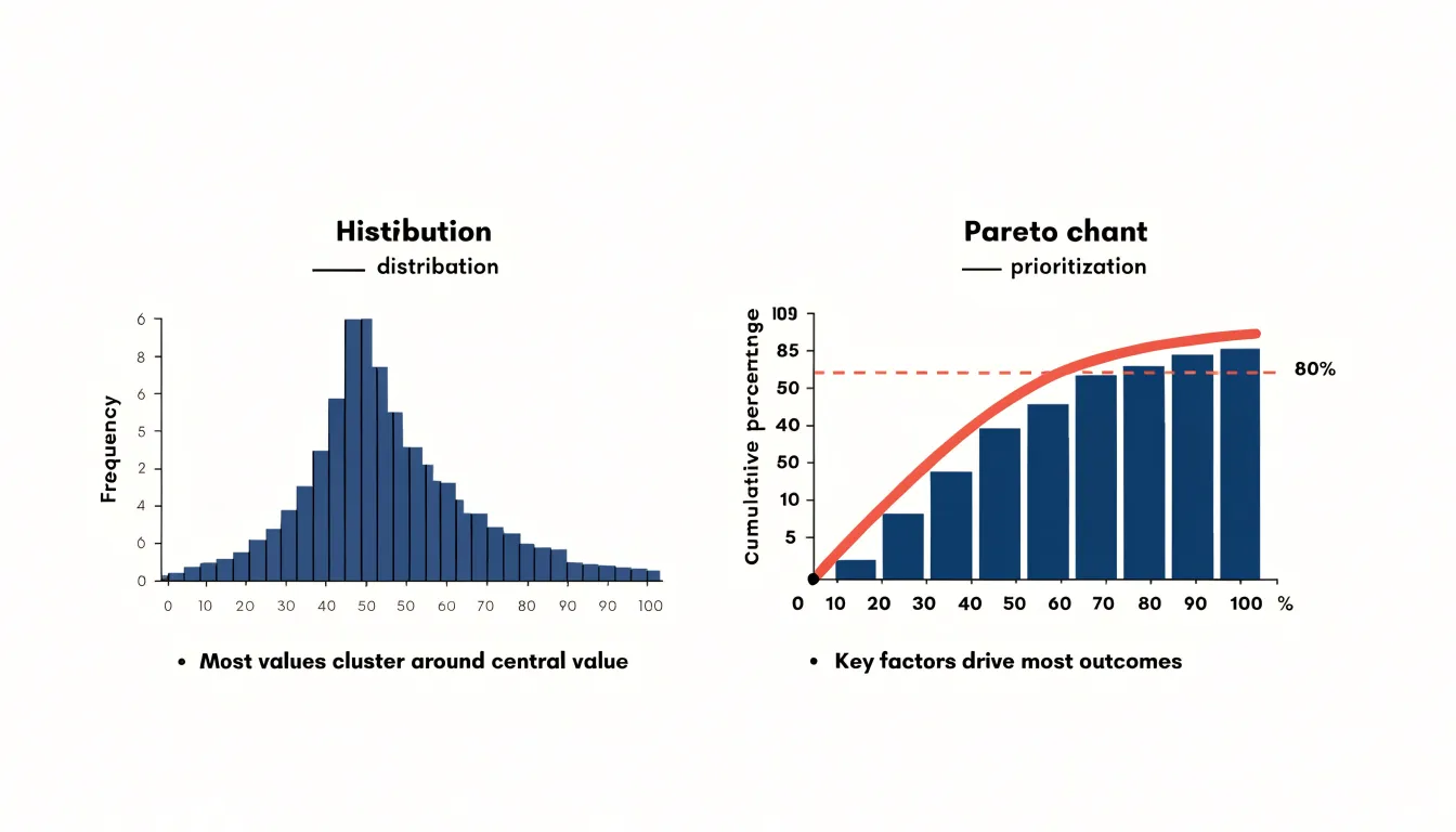
Table of Contents
Histogram
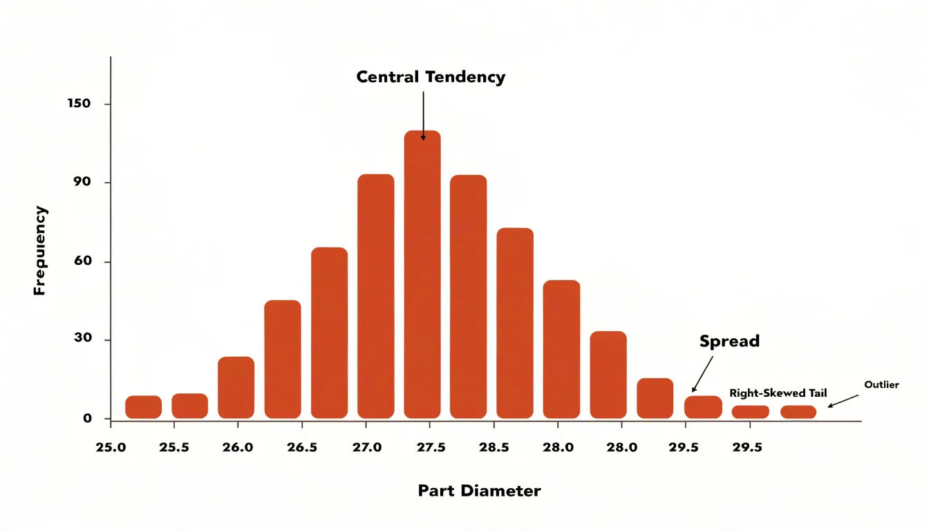
A histogram provides a visual summary of how continuous quantitative data distributes across a range of values. The data is divided into equal-interval bins, sometimes called classes, spanning from the smallest to the largest observation. Each bin is represented by a vertical bar whose height corresponds to the frequency, or count, of observations within that interval. Because the intervals are equal in width and adjacent with no gaps, the bars form a continuous profile that mirrors the underlying distribution.
Choosing the number and width of the bins shapes how much detail the chart reveals. Too few bins compress the data into a coarse block that hides subtle variation, while too many produce a fragmented picture dominated by noise. A balanced bin width allows underlying patterns to emerge, including central tendency, the spread of values around that center, and clusters where observations concentrate. Analysts can also identify skew, where the distribution stretches toward one tail, and multimodal shapes where two or more distinct peaks appear, each suggesting different subgroups within the data.
Because the bars are equal in width, the area of each bar is proportional to the number of observations in its interval, and the total area reflects the full dataset. This property makes histograms useful for comparing distributions across groups and for spotting outliers that sit far from the main body of data. When a histogram shows a smooth, bell-like shape, the data behaves predictably around its mean. Sharp peaks or long tails signal that the underlying process may warrant closer investigation to determine where variation originates.
Pareto Chart
A Pareto chart ranks categorical factors by their frequency or severity so that the most consequential inputs appear first, showing teams where attention will yield the greatest return. The chart combines a bar graph, with categories arranged in descending order of impact, and a cumulative percentage line that tracks how quickly the running total approaches the full count. Named for Vilfredo Pareto, whose observations about wealth distribution inspired the principle later popularized by Joseph Juran as the “vital few and the trivial many,” the chart rests on the empirical regularity that a small subset of causes typically produces the majority of effects.
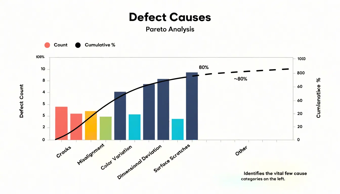
Building one begins with collecting data on a categorical variable such as defect type, complaint source, or machine stoppage reason. Counts are sorted from largest to smallest and drawn along the horizontal axis, with frequency or cost on the vertical axis and a cumulative percentage line overlaid. The steepness of that line identifies the vital few on the left side that accumulate most of the total. A common convention is to mark the point where the cumulative curve crosses roughly 80 percent, though the exact threshold should be set by practical judgment rather than treated as fixed.
The severity dimension matters as much as raw frequency. A defect type that occurs rarely but carries high cost, safety risk, or customer impact may deserve priority over more common but trivial issues, so the ranking metric can be weighted counts, rework hours, or financial loss. This flexibility makes the chart useful in quality improvement, maintenance planning, and service operations. Once the vital few are identified, improvement efforts can be scoped tightly around them, and the chart can be redrawn after changes are made to verify that the ranking has shifted.
Visual Structure
A histogram is built around a single horizontal axis carrying a continuous scale of values. Bars sit flush against one another to signal that the intervals connect without gaps, so readers scan the bars as one continuous silhouette rather than as separate categories.
A Pareto chart arranges its categorical bars in descending order from left to right and plots its cumulative percentage line against a second vertical axis, typically scaled from 0 to 100 percent, while the primary vertical axis carries the raw counts or costs. The two axes share the same horizontal categories, yet they measure different quantities, so the line and the bars must be read in relation to their respective scales. This dual-axis setup lets viewers see both the size of individual contributions and how quickly the cumulative total approaches completeness. The line rises steeply at first and flattens as smaller categories accumulate, forming a layered visual that directs attention from the tallest bars toward the cumulative threshold.
Data Types
The distinction between the two charts begins with the input data each is designed to receive. A histogram works with continuous numeric variables—measurements that can take on any value within a range and be subdivided indefinitely, such as order processing time, product weight, furnace temperature, or the diameter of a machined part. Because bins are intervals along a number line, their order is fixed by magnitude rather than by the analyst’s judgment.
A Pareto chart operates on discrete categorical labels that name something rather than measure it, such as defect types, complaint categories, machine identifiers, or supplier names. Because qualitative buckets have no inherent numeric order, the Pareto chart deliberately sorts the bars from most to least frequent.
The input data must match the chart. Passing continuous measurements to a Pareto chart requires collapsing them into arbitrary categories, which discards the detail a histogram preserves. Conversely, categorical labels have no natural numeric position along an axis, so binning them into a histogram makes little sense.
The 80/20 Rule
The 80/20 Rule describes a recurring pattern in which roughly 80 percent of problems stem from 20 percent of causes. Originating from Vilfredo Pareto’s observation that a minority of the population held the majority of the land and later applied to process failures by Joseph Juran, this ratio serves as a practical heuristic rather than an exact law. While the precise split varies by context, the underlying imbalance is consistent across manufacturing, service operations, and administrative processes.
Within quality management, the rule helps teams prioritize when the raw volume of defects, complaints, or delays appears overwhelming. A production line might find that a few specific fault types generate the majority of scrap, or a support desk might discover that a small set of recurring questions consumes most of its handling time. Rather than attempting to address every contributing factor simultaneously, teams focus on the few causes with the greatest leverage to produce faster reductions in waste and rework.
Applying the 80/20 Rule requires reliable data on causes and their frequencies, along with a willingness to revisit the analysis. Because improvements shift the distribution, what was once a vital few will change, making the rule a repeatable habit of prioritization rather than a one-time finding.
Frequency and Bins
By grouping a long list of continuous measurements into range-based intervals—for example, 10 to 20 units, 20 to 30 units, and so on—a histogram makes patterns visible that would be hidden in a raw data table. Analysts often experiment with several bin widths to find a balance that suits the data and the question at hand.
Once the bins are drawn, three features become immediately readable:
- Central tendency shows up as the location of the tallest bars, indicating where most observations cluster.
- Spread appears in how far the bars extend to the left and right, showing the range and variability of the measurements.
- Skewness emerges from the asymmetry of the profile, with a long tail on one side signaling that extreme values pull the distribution in that direction.
Because the histogram depends on grouped frequencies rather than individual points, it serves as a natural bridge between raw observations and the summary statistics that describe them, helping analysts decide whether further statistical testing is warranted.
Sorting and Cumulative Lines
Sorting a Pareto chart’s categories so that each subsequent bar is equal to or shorter than the one before it forces attention onto the largest contributors first. A reader can scan from left to right and see impact diminish bar by bar.
Across the tops of the bars, the cumulative percentage line is plotted at each point where a running total is reached. The running total is calculated by adding each category’s value to the sum of all categories to its left, then dividing that sum by the grand total. The cumulative line therefore starts at the first bar with that category’s own share, climbs steeply through the first few categories, flattens as smaller categories are added, and ends at 100 percent at the rightmost bar. The point where this line crosses a chosen threshold (such as 80 percent) isolates the categories to the left as the primary targets for improvement work.
Quality Control
In manufacturing and operations, Pareto charts help quality engineers sort competing defect types, rejections, and customer complaints. On a production line making machined parts, for example, a chart might reveal that three defect types—dimensional out-of-tolerance, surface scratches, and thread damage—together represent nearly 80 percent of all scrap. That finding lets the team set aside lower-volume issues and concentrate inspection, tooling adjustments, and operator training on the categories driving the greatest loss.
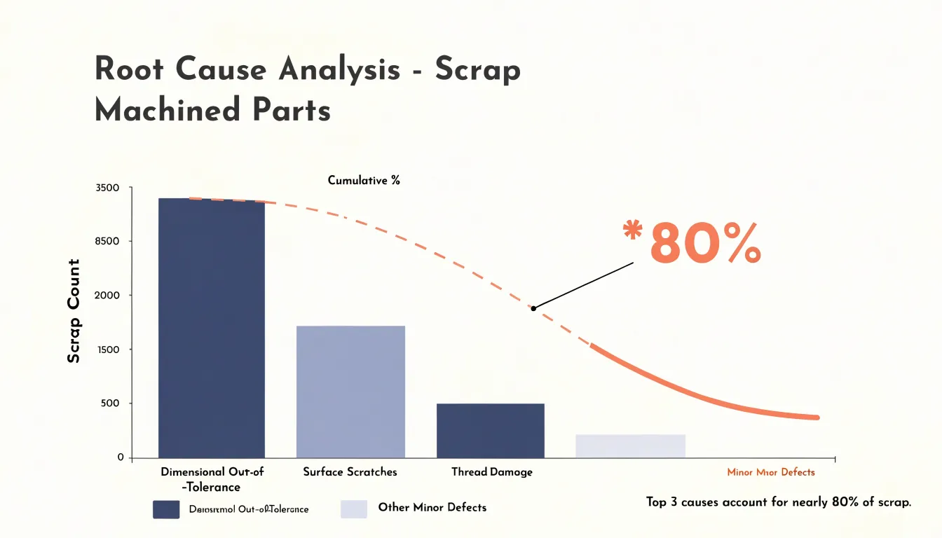
The chart also narrows the scope of root cause analysis. Rather than convening a cross-functional team to examine every possible failure mode, facilitators can direct a fishbone diagram or five-whys session at the top-ranked defect category, where improvements translate into measurable gains in yield and cost. Used as a before-and-after tool, teams implement corrective actions on the leading categories and re-plot the data after a few weeks to confirm those categories have shrunk and to identify the next tier of problems.
Effective application requires reliable defect classification, consistent recording by operators and inspectors, and regular chart updates so the analysis reflects current conditions and demonstrates the impact of quality initiatives to management.
Process Variation
Reading a histogram’s shape gives teams a fast diagnostic for process stability before any formal statistical test is applied:
- Normal (bell-shaped): Signals a stable process dominated by many small, common causes that balance each other out, with most readings near the average.
- Skewed: A long tail stretching to the left or right often points to a natural boundary the process presses against (such as a measurement that cannot fall below zero) or a skewing influence like rework, sorting, or a drift in machine settings.
- Bimodal: Two distinct peaks usually mean two different conditions are mixed in one dataset—such as output from two shifts, two machines, two suppliers, or two operator methods—exposing hidden instability that simple averages obscure.
- Outliers, truncated, or flat shapes: Isolated bars far from the main cluster indicate outliers; data bunching abruptly at a limit shows a truncated distribution; and flat, uniform shapes suggest several sources blended together.
By comparing histogram shapes across time periods, shifts, or subgroups, teams can confirm whether a process is stable or drifting.
Choosing the Right Chart
Selecting between the two charts depends on the analytical question and the criteria of your dataset.
Use a histogram when:
- You have a continuous variable measured on a consistent numerical scale (such as cycle times, fill volumes, or tensile strength).
- Your sample size is large enough to populate the bins meaningfully.
- You need to answer questions about process behavior in a single snapshot, such as whether a process meets specification, how much variation exists, or whether the distribution is symmetric.
Use a Pareto chart when:
- You have categorical count data (or weighted impact metrics) organized under a meaningful classification scheme.
- You need to rank discrete failure modes or complaint reasons to decide which problem deserves resources first.
In practice, the two tools often work as complements: a Pareto chart identifies the dominant defect category, and a histogram then examines the continuous measurements associated with that category to understand its underlying distribution.
Real World Scenarios
Quality assurance teams frequently rely on both charts in sequence during continuous improvement projects:
- Prioritize with a Pareto chart: Faced with elevated defect rates, a manufacturing team collects a month of inspection records, tallies occurrences by defect type, and plots a Pareto chart. The chart reveals which few defect categories account for the majority of issues.
- Diagnose with a histogram: Focusing on the top-ranked defect category, the team gathers continuous process measurements (such as dimensional readings, cycle times, or weights) and plots a histogram. The distribution’s shape, center, and spread reveal whether output clusters around a target, skews toward a specification limit, or displays multiple peaks from mixed inputs, helping locate the source of variation.
- Verify improvements: After implementing corrective changes, the team collects fresh data and rebuilds both charts. The new Pareto chart confirms that the targeted defect category has shrunk and reveals the new leading category, while the updated histogram verifies that the measurement distribution has tightened and shifted toward the target.
Common Pitfalls
Choices about scales and setups can distort how both charts are interpreted:
- Inappropriate bin width (Histogram): Too few bins make data appear more uniform than it is, while too many create a spiky chart that obscures trends. Verify that the bin width fits the data range and sample size.
- Biased bin starting points (Histogram): The starting point of the first bin can shift the visual impression of the distribution and should be chosen thoughtfully.
- Improper dual-axis scaling (Pareto chart): If the secondary percentage axis is not scaled and aligned to match the primary count axis, the cumulative line may fail to reach 100% at the final bar, reach 100% prematurely, or cross bars at misleading points, distorting the true contribution of each category.
- Unsorted bars (Pareto chart): Failing to sort the bars in descending order defeats the purpose of the Pareto principle.
Interpreting Results
Interpreting results means converting visual patterns into concrete operational choices, each ending with a named owner, a defined next action, and a follow-up measurement point. Documenting the reasoning behind each conclusion allows teams to refine their interpretation as new data arrives.
When reading a histogram:
- A distribution pressed against a specification limit signals that a meaningful share of output risks falling out of tolerance. Next actions include centering adjustments, tighter process controls, or reviewing the specification itself.
- A long tail or isolated outliers direct attention to intermittent causes such as setup changes, raw material batches, or operator variation. Next actions include adjusting a machine setting, scheduling additional inspection, or collecting a short run of fresh data to confirm the pattern.
When reading a Pareto chart:
- Categories making up roughly the first 80 percent of the cumulative total receive active corrective effort, while the remaining trivial many are simply monitored, freeing resources for high-leverage work.
Final Checklist
Before committing to a chart type, run through these ten questions:
- What is the goal of the analysis? Are you prioritizing causes (Pareto) or showing a distribution of measurements (histogram)?
- What is the nature of the data? Is it categorical groups (Pareto) or continuous values along a range (histogram)?
- How should bars be ordered? Do you need bars sorted from largest to smallest to highlight the vital few (Pareto), or ordered sequentially by value to reveal shape (histogram)?
- Do you need a cumulative line? Include a secondary cumulative percentage line for a Pareto chart; omit it for a histogram.
- What question will your audience ask? Use a Pareto chart if they ask which category contributes most; use a histogram if they ask how values are spread.
- Does the data meet the chart’s assumptions? Ensure you have countable occurrences (or costs) per category for a Pareto chart, or a sufficient sample of numeric data for a histogram.
- How much visual space is available? Many categories can clutter a Pareto chart, and too many bins can obscure patterns in a histogram.
- Is the grouping fixed or adjustable? Pareto charts use fixed qualitative categories, whereas histograms require you to adjust bin widths to set the level of detail.
- Do you need to compare across groups? Both charts can be split by subgroup (such as shifts or machines), though doing so adds visual complexity.
- What is the operational outcome? Use a Pareto chart to scope and target a problem; use a histogram to understand and center a process.
Frequently Asked Questions
What is the difference between a Pareto chart and a histogram?
A histogram shows how continuous quantitative data is distributed across equal-interval bins, while a Pareto chart ranks categorical factors by frequency or severity and adds a cumulative percentage line. In practice, a Pareto chart can identify the dominant defect category and a histogram can then examine the continuous measurements associated with that category.
When should I use a histogram instead of a Pareto chart?
Use a histogram when you have a continuous variable measured on a consistent numerical scale and a sample large enough to populate the bins meaningfully. It helps answer questions about process behavior in a single snapshot, such as how much variation exists or whether the distribution is symmetric.
When should I use a Pareto chart?
Use a Pareto chart when you have categorical count data or weighted impact metrics organized under a meaningful classification scheme. It is used to rank discrete failure modes or complaint reasons so you can decide which problem deserves resources first.
How do you read a histogram’s shape?
A histogram’s tallest bars indicate central tendency, the bars’ left-to-right extent shows spread, and a long tail on one side signals skewness. Two distinct peaks can indicate two different conditions mixed in one dataset, and isolated bars far from the main cluster indicate outliers.
What does the 80/20 rule mean in a Pareto chart?
The 80/20 Rule describes a recurring pattern in which roughly 80 percent of problems stem from 20 percent of causes, but it is a practical heuristic rather than an exact law. A common convention is to mark where the cumulative curve crosses roughly 80 percent, though the exact threshold should be set by practical judgment.
Can a rare defect be prioritized on a Pareto chart?
Yes. The severity dimension matters as much as raw frequency, so a defect type that occurs rarely but carries high cost, safety risk, or customer impact may deserve priority over more common but trivial issues, and the ranking metric can be weighted counts, rework hours, or financial loss.
Tony Astor
Tony writes about data visualization and the tools people use to build charts and dashboards. More about Data Illustrator