Pareto Chart: How to Apply the 80/20 Rule Visually
 By Tony Astor ·

Pareto Chart
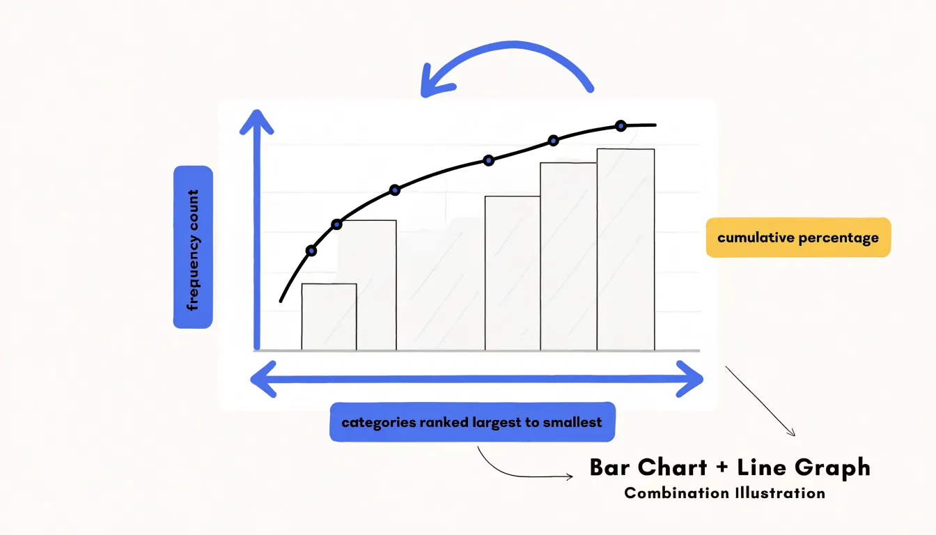
A Pareto chart is a bar-and-line graph that ranks categories from largest to smallest, with bars showing each category’s frequency and a line tracking cumulative percentage. Named for Vilfredo Pareto, it applies the 80/20 principle to reveal the “vital few” categories causing most of a problem, helping teams prioritize improvement efforts.
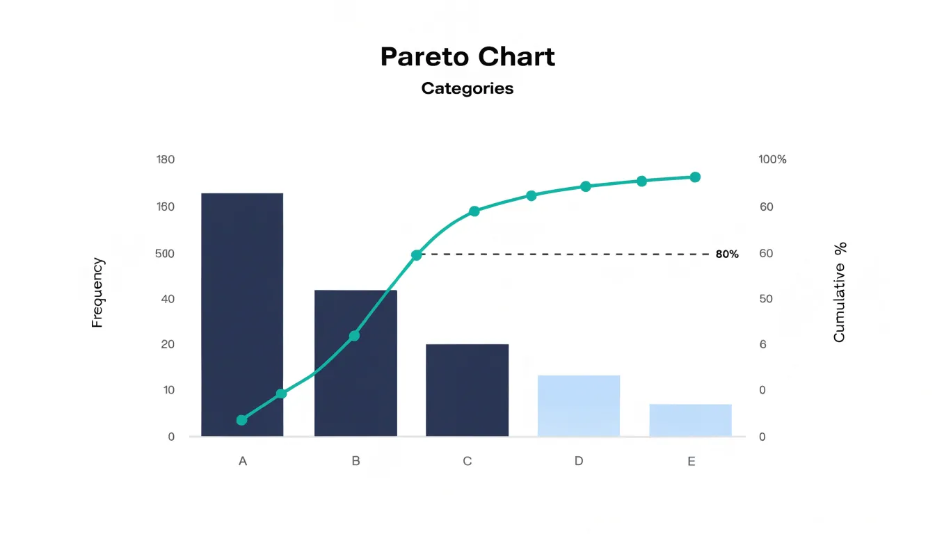
Table of Contents
Pareto Chart
The Pareto chart is a specialized bar-and-line graph that combines frequency counts with cumulative percentages on a single display. Vertical bars represent individual categories, arranged from tallest to shortest along the horizontal axis, while a second vertical axis carries a cumulative percentage line. This dual-axis arrangement ties raw magnitude to proportion, letting a reader see at a glance which handful of categories account for the bulk of the total. The chart is named for Vilfredo Pareto, the Italian economist whose observations about wealth distribution led to the broader principle now known as the 80/20 rule: roughly 80% of outcomes stem from 20% of the contributing causes.
To construct the chart, an analyst counts occurrences for each category, ranks them in descending order, and computes a running total expressed as a percentage of the grand total. The bars show each category’s absolute contribution, and the line climbs from left to right, tracking how much of the whole has been accounted for as each successive category is added. The point where the line crosses the 80% mark identifies the “vital few” categories that drive most of the effect. The remaining categories, sometimes aggregated into an “other” bar, form the “trivial many.”
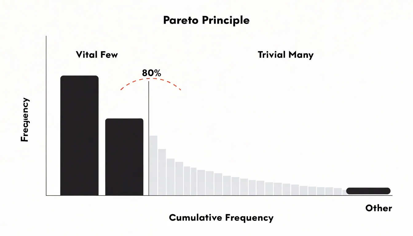
The 80/20 ratio describes a general tendency rather than a fixed law. Real data rarely lands on 80 and 20; a given process may show that 78% of complaints come from 15% of defect types, or that 90% of delays trace to 22% of causes. The chart’s value lies in making that concentration visible and measurable, turning a list of problems into a prioritized improvement agenda.
Pareto Chart
The method behind the Pareto chart traces back to Vilfredo Pareto, an Italian economist and sociologist working in the late nineteenth and early twentieth centuries. While studying the distribution of wealth in Italy, Pareto observed a striking imbalance: a relatively small proportion of the population held the majority of the wealth. He documented this pattern across different countries and time periods, finding it remarkably consistent. Over time, others extended and formalized his insight into the conceptual foundation for the prioritization technique that bears his name.
The transition from Pareto’s economic observations to a practical analytical tool came through its graphical format. Human cognition has real limits when processing many discrete data points at once. A table of dozens of defect categories, each with its own count, demands effortful comparison and mental arithmetic to rank and total. A Pareto chart performs that work visually, reducing the cognitive load required to identify which inputs account for most of the outcome.
The eye is drawn to the few tallest bars on the left, while the cumulative line shows precisely where the curve begins to flatten. Observers can see the dominant contributors, grasp their relative weight, and locate the threshold of diminishing returns in a single glance, allowing attention to move quickly toward investigation and action.
Data Collection
Effective Pareto analysis begins with disciplined data collection. Raw inputs—incident reports, customer complaints, production logs, or defect records—must be captured consistently so the resulting chart reflects reality. Start by defining the scope and time frame clearly. For example, if analyzing product defects, decide whether to include all production lines or a specific shift, and set a fixed period such as the last quarter. This prevents mixing data from different contexts that could distort the distribution.
Next, establish a reliable capture method. Automated systems like error trackers or CRM tickets reduce human error, but manual logs can work if standardized. Train staff to record each occurrence with consistent fields: date, type, location, and description. Use unique identifiers to avoid duplication. For baseline metrics, consider both frequency (how often an issue occurs) and impact (cost, downtime, or severity).
After collection, group the data into distinct, actionable buckets. Too many categories dilute the concentration effect, while too few obscure root causes. Start with natural groupings—by defect type, failure mode, or customer complaint category—and refine them:
- Aim for 5–10 categories for clarity.
- Ensure buckets are mutually exclusive and collectively exhaustive so every data point fits one category.
- Merge rare categories into an “other” bucket only if they are truly negligible; otherwise, keep them separate for analysis.
- Use consistent naming conventions for recurring issues and periodically review the taxonomy to adapt to new patterns.
Finally, validate the data. Cross-check a sample against source records and look for missing entries or outliers. Clean the dataset by resolving duplicates and correcting misclassifications, and document the collection and grouping process so others can replicate or audit it.
Frequency Counts
Frequency counts form the quantitative backbone of a Pareto analysis, converting raw observations into a ranked picture of where effort will pay off most. The counts should be gathered over a defined window, since short samples can overstate rare events while long windows smooth out seasonal distortion. Analysts typically choose among three counting methods depending on the nature of the problem:
- Straight occurrence counts: Each time a defect, complaint, or failure mode appears, it is tallied. This works well when every occurrence carries roughly equal consequence, such as the number of customer tickets per issue type or the count of machine stoppages by cause.
- Occurrence rates: Instead of asking how many times an issue happened, the analyst asks how often it happens per unit of opportunity: per thousand units produced, per hundred transactions, per month of machine operation, or per employee. Normalizing against exposure makes categories comparable even when their underlying volumes differ, revealing whether a high count reflects genuine severity or simply a high-volume process. Rate calculation requires capturing both the event and a reliable exposure denominator over the same period.
- Financial cost: Weighting each category by monetary impact can reorder a ranking entirely, elevating a modest number of expensive failures above a large number of trivial ones. Direct costs are usually the easiest to assemble: scrap value, rework labor, warranty payouts, refunds, or replacement parts. Indirect costs—lost production time, expedited shipping, or staff hours spent on escalated complaints—demand more estimation but often dominate the total. Multiplying each category’s count by its average cost per occurrence produces a cost-weighted frequency.
Whichever method is chosen, consistent definitions and clean data matter more than sophistication. Document how each category is counted, verify totals against source systems, and check that the chosen metric aligns with the decision the chart is meant to support.
Ranking
Before any bars are drawn or axes labeled, the underlying data table should be sorted from the largest count or cost down to the smallest. This descending arrangement places the dominant contributor at the top of the table and the trivial contributors at the bottom, creating an instant visual hierarchy even in plain text. Because the top rows accumulate quickly toward the majority of the total while the tail rows contribute little individually, sorting in this direction ensures that cumulative percentages rise steeply at the start and flatten toward the end.
Pre-sorting the data table also provides several practical benefits for plotting and review:
- Automated chart order: Plotting software typically preserves the row order of the source table, so a pre-sorted table yields a chart whose bars descend smoothly from left to right without manual adjustment.
- Cross-reference clarity: Consistency between table and chart prevents confusion when stakeholders review both together.
- Tie resolution: Sorting exposes ties and near-ties among categories, prompting analysts to decide how to handle equal values before the graphic freezes those decisions.
- Data scrutiny: A ranked table makes it easier to verify outliers at the top and identify long tails at the bottom that should be grouped into an “other” category.
Cumulative Percentage
The cumulative percentage is the running total that turns a ranked bar graph into a diagnostic tool. Moving bar by bar from left to right, each point on the cumulative line shows the share of total impact accounted for by all categories up to that position. To calculate it, divide each category’s value by the grand total to get its individual share, then keep a running sum of those shares in ranked order. The first point equals the largest category’s own percentage; the second equals the first plus the second; and the final point reaches 100 percent.
This running sum allows you to locate the cutoff point with precision. Rather than estimating by eye where the vital few end and the trivial many begin, you read along the cumulative line until it first crosses the 80 percent mark. In practice the line rarely lands exactly on 80, so you note the category where the line crosses the threshold and count how many categories fall at or before it. That count defines the scope of your improvement effort, telling you how many contributors to address before diminishing returns set in.
Bar Chart
The bar chart forms the primary layer of a Pareto display, showing each category’s contribution as a solid vertical bar rising from the horizontal axis. The tallest bar appears on the far left, and each bar’s height corresponds to the raw count, rate, or cost read from the left-hand vertical axis. This left axis is scaled to accommodate the highest value so the tallest bar fits comfortably within the chart area.
The bars are typically drawn with uniform width and spacing, creating a clean, comparable series. In practice, they are often color-coded or shaded to distinguish them from the cumulative line overlaid on the right axis. Even without that line, the sorted bar chart stands on its own as a straightforward comparison of initial relative sizes.
Line Overlay
The line overlay transforms the sorted bar chart into a complete Pareto chart. A second vertical axis is added on the right-hand side, scaled from 0 to 100 percent, and the running total of percentage shares is plotted as a line of connected points, one per category.
Because the categories are sorted from largest to smallest, the cumulative line rises steeply at first and flattens out as smaller contributors are folded in. A small bar with a high percentage share pushes the line up sharply, while a bar with a modest share barely moves it. A reader can trace the line from left to right to see how much of the total problem is captured after two, three, or four categories, while the steepness of the early segments communicates how concentrated the effects are. Marking the individual points on the line, labeling the right axis clearly, and adding a horizontal reference line at the 80 percent level keep the overlay easy to read.
Vital Few
Separating the “vital few” categories from the long tail of minor contributors is the central analytical task of Pareto analysis, because it determines where improvement effort will produce the greatest return. The value of this step lies in the discipline it imposes on resource allocation. Without it, teams tend to respond to the most recent or most visible problem rather than the most consequential one. With a clear vital few list, improvement resources—whether engineering time, maintenance budgets, or process redesign effort—flow toward the handful of categories with the highest leverage.
This focus also produces faster feedback. When a team concentrates on two or three dominant drivers, the effect of each fix becomes visible in the data within a short cycle, which sustains momentum and builds confidence in the method. Documenting which categories were classified as the vital few, along with the thresholds used to decide, keeps the analysis transparent. Because the vital few are not a permanent designation, they will shift as major problems are resolved and new ones emerge.
Trivial Many
The “trivial many” represent the long tail of factors that remain once the vital few have been identified—often roughly 80 percent of the categories, each accounting for only a fraction of the total effect. Individually these issues appear manageable, and teams often address them because they are visible, familiar, or easy to resolve. Taken together, however, they consume a disproportionate share of time, attention, and resources while producing minimal movement in overall performance.
Filtering out the trivial many is a deliberate act of prioritization. Once separated, these minor items can be set aside, deferred, or monitored without immediate action. The discipline lies in resisting the temptation to chase every small imperfection, especially when quick wins on minor items create an illusion of progress.
Isolating these minor factors also has diagnostic value. Grouping them clarifies how much collective effort they absorb, which can justify decisions to streamline processes, automate handling, or simply accept a certain level of imperfection. It shifts the conversation from resolving every individual complaint to managing the overall portfolio of issues.
The trivial many should not be discarded permanently. They serve as a holding area for low-priority work; as major causes are resolved, the distribution of problems changes, and some previously minor factors may grow in relative importance during periodic re-analysis.
Everyday Use
Beyond business analytics, the Pareto chart can be applied to personal habits, productivity, and wellness. Start by tracking your daily routines for a week: log each activity, the time spent, and the perceived benefit. Categorize these activities and plot them to see which habits contribute most to your productivity or well-being.
For instance, you might find that a 30-minute morning planning session dramatically improves your focus, while hours spent on email yield little. In health, you can chart the factors that most affect your energy or mood—such as sleep quality, nutrition, or exercise—and prioritize those. This helps you avoid the trap of over-optimizing low-impact areas. By re-charting after adjusting your routine, you can track shifts in your personal vital few over time.
Business Use
In business settings, Pareto charts give managers a shared visual anchor for triage, ownership, and measuring whether an intervention moved the biggest bar:
- Customer service: Support organizations often log incoming tickets by category over a quarter. Case studies frequently show that a handful of issues—such as password resets, billing questions, and delivery tracking—account for the vast majority of volume. Addressing the top category with a self-service help article or an automated reset flow cuts contact volume without touching the long tail of rare requests.
- Inventory control: By charting the causes of stockouts or the frequency of slow-moving items, a warehouse can see which small set of SKUs drives most holding costs or missed shipments. A retail store, for example, can reduce dead stock by reordering only the 20 percent of items that generate most of the revenue and shrinking shelf space for the rest.
- Quality assurance: Manufacturers tally failures by defect type and line location. Studying warranty returns might reveal that one component family produces most failures, focusing engineering analysis on that component instead of spreading effort across every possible fault.
Common Mistakes
Several recurring errors in construction and interpretation can undermine the conclusions drawn from a Pareto chart:
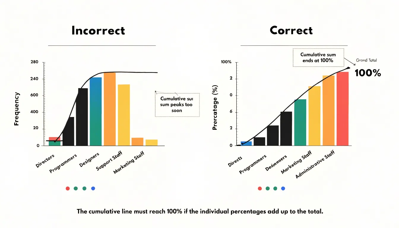
- Improper scale alignment: When the frequency axis on the left and the cumulative percentage axis on the right do not share a consistent reference point, the bars and the rising line can tell contradictory stories. If the cumulative curve peaks too early or the 80 percent threshold appears at an implausible position, check the axes. Aligning the cumulative axis so that 100% matches the grand total on the bar axis keeps the visual comparison honest.
- Poor data grouping: Categories that are too broad bury meaningful variation, while categories sliced too finely scatter small counts across many bars and flatten the visible contribution of a dominant factor. Similarly, an oversized “other” bar can mask a cluster of related causes that deserve their own category. Review category definitions against the raw data before charting to ensure each bar represents a coherent, comparable unit of analysis.
- Confusing ranking with causation: A Pareto chart shows where problems concentrate, not why they occur. Teams sometimes jump directly from the chart to a corrective action aimed at the top bar without confirming whether that category is a genuine driver or merely correlated with the outcome. Treat the diagram as a prioritization tool rather than causal proof.
Root Cause Analysis
Because prioritization without diagnosis leads to superficial fixes, a Pareto chart is most effective when paired with root cause analysis. Once the chart identifies which categories account for most of the impact, deeper investigation begins with tools like the 5-Why method and the Fishbone diagram.
The 5-Why analysis works by repeatedly asking why a problem occurs, tracing a visible symptom back through intermediate conditions until the team reaches a correctable process failure. A Fishbone diagram complements this by organizing potential causes into structured categories—people, methods, machines, materials, measurement, and environment—so the team can brainstorm and test hypotheses systematically rather than jumping to the first plausible explanation.
Used together, these tools distinguish symptom from cause. A machine that stops frequently may appear as the tallest bar on a Pareto chart, while the Fishbone and 5-Why investigation reveal that inconsistent incoming material or a skipped maintenance step is actually driving the stoppages. Anchoring each Pareto priority to a documented root cause ensures corrective actions target the underlying process, preventing the same category from returning to the top of the next chart.
Dashboard
Once a Pareto-driven improvement has been implemented, a continuous monitoring dashboard helps sustain the gains. The dashboard should be designed around the specific categories or defect types identified in the original analysis, so each bar or trend line corresponds directly to a cause the team chose to act on.
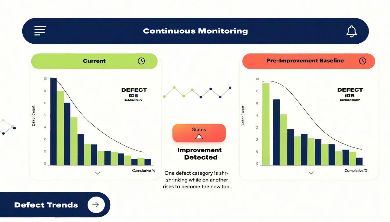
Reviewing the dashboard on a regular cadence turns it into an active management tool:
- Compare against baseline: Check current performance against pre-implementation numbers to confirm whether targeted categories have shrunk as expected.
- Spot early warning signs: Watch for metrics that drift back toward previous levels, indicating that an underlying cause was not fully addressed or that a process control has slipped.
- Identify the next priority: When a leading category falls away, a live dashboard makes the reordering visible immediately without requiring a fresh data-collection exercise, allowing the team to redirect effort toward the new top contributor.
Frequently Asked Questions
What is a Pareto chart?
A Pareto chart is a specialized bar-and-line graph that combines frequency counts with cumulative percentages. Its vertical bars are arranged from tallest to shortest, and a cumulative percentage line on a second vertical axis shows how much of the total is accounted for as categories are added.
How do you make a Pareto chart?
To build one, count occurrences for each category, rank the categories in descending order, and compute a running total expressed as a percentage of the grand total. The bars show each category’s absolute contribution, while the line climbs from left to right.
What does the 80/20 rule mean in a Pareto chart?
The 80/20 rule is the broad principle that roughly 80% of outcomes stem from 20% of contributing causes. The article notes this is a general tendency, not a fixed law, and real data rarely lands exactly on 80 and 20.
What is the cumulative percentage line on a Pareto chart?
The cumulative percentage line is a running total showing the share of total impact accounted for by all categories up to that point. To calculate it, divide each category’s value by the grand total, then keep a running sum of those shares in ranked order until the final point reaches 100 percent.
What are the vital few and trivial many in Pareto analysis?
The vital few are the categories at or before the point where the cumulative line first crosses the 80% mark, representing the contributors that drive most of the effect. The trivial many are the remaining long-tail factors, often roughly 80% of the categories, each accounting for only a fraction of the total.
How is a Pareto chart used with root cause analysis?
Once a Pareto chart identifies the categories accounting for most of the impact, it can be paired with root cause analysis tools like the 5-Why method and Fishbone diagram to investigate deeper. The chart is a prioritization tool, not causal proof, so it shows where problems concentrate rather than why they occur.
Tony Astor
Tony writes about data visualization and the tools people use to build charts and dashboards. More about Data Illustrator