Parallel Coordinates Plot: Visualizing Multivariate Data
 By Tony Astor ·

Parallel Coordinates Plot
A parallel coordinates plot is a multivariate visualization that places each variable on its own vertical axis, with every data record drawn as a polyline crossing all axes at its values. It reveals correlations, clusters, and outliers across many attributes in one view, overcoming the scaling limits of scatter plots.
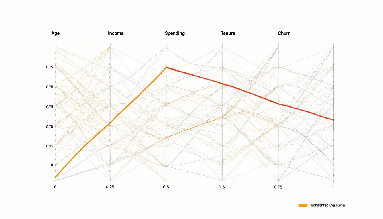
Table of Contents
- Parallel Coordinates Plot
- Parallel Coordinates Plot
- Parallel Coordinates Plot
- Parallel Coordinates Plot
- Parallel Coordinates Plot
- Parallel Coordinates Plot
- Parallel Coordinates Plot
- Parallel Coordinates Plot
- Parallel Coordinates Plot
- Parallel Coordinates Plot
- Parallel Coordinates Plot
- Parallel Coordinates Plot
- Parallel Coordinates Plot
- Parallel Coordinates Plot
- Parallel Coordinates Plot
Parallel Coordinates Plot
A parallel coordinates plot arranges each variable in a dataset as its own vertical axis, placing the axes side by side so that a single record becomes a polyline crossing every axis at its corresponding value. This structure lets an analyst follow one data instance across dozens of attributes at once, reading a customer, a patient, or a machine part as a continuous trajectory from left to right. Each line carries the full profile of that instance, and the collective bundle of lines carries the shape of the entire dataset. Where a traditional scatter plot is limited to two or three dimensions, this layout scales to ten, twenty, or more attributes without multiplying the number of charts an analyst must inspect.
Correlations, clusters, and outliers surface directly from the geometry:
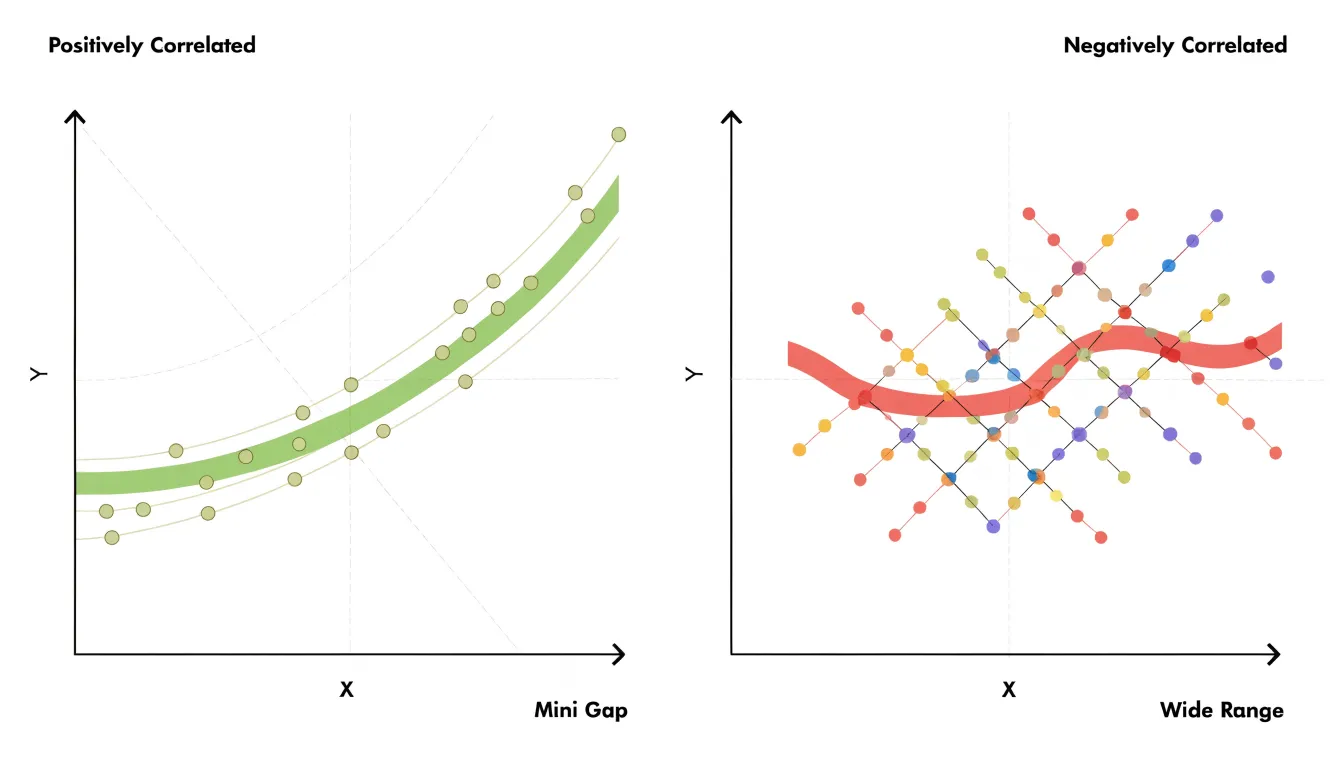
- Positive relationships between two adjacent axes appear as lines running roughly parallel or converging into a tight band.
- Inverse relationships appear as lines crossing in a dense braid between the two axes.
- Clusters emerge as distinct strands or bundles that separate from the main mass, revealing subgroups defined by combinations of attribute values rather than by any single field.
- Outliers appear as lines that spike away from their neighbors on one or more axes.
Non-adjacent variables can be compared by following lines across the intervening axes, and analysts often reorder axes to place variables of interest side by side. Analysts can also apply brushing, selecting a range on one axis to highlight only the lines passing through it, which then trace how that subgroup behaves across all remaining attributes. The result is a compact visual summary in which global structure and individual records coexist in the same view.
Parallel Coordinates Plot
Traditional scatter plots visualize relationships between two variables, and 3D scatter plots add depth for a third. However, as the number of variables grows, these approaches become impractical. A scatter plot matrix, which arranges pairwise scatter plots in a grid, offers a common workaround for exploring multiple variables. Yet the number of pairwise plots grows quadratically with the number of variables: for $n$ variables, an $n \times n$ grid is required. With just ten variables, that means 45 distinct pairwise plots (excluding the diagonal), and with twenty variables, it balloons to 190.
This exponential explosion overwhelms both screen real estate and human cognition. Each plot competes for limited display space, forcing viewers to shrink plots to the point of illegibility or scroll through endless panels, losing the holistic view. Moreover, the cognitive load of mentally stitching together patterns across dozens or hundreds of plots makes it difficult to detect higher-order interactions or multivariate trends.
Parallel coordinates plots overcome these limitations by packing all variables into a single display that fits within the screen, eliminating the need for multiple panels. Instead of comparing many separate scatter plots, the viewer reads the crossings and slopes of lines across a fixed set of parallel axes, making the chart a staple in exploratory data analysis and multivariate visualization.
Parallel Coordinates Plot
In a parallel coordinates plot, the vertical axes stand side by side as evenly spaced parallel lines. Each axis is scaled independently to the range of the variable it represents, so the minimum value sits at the bottom of the axis and the maximum at the top, with intermediate values distributed proportionally along the vertical span. This independent scaling gives every variable the full height of the plot, keeping the geometry of each axis comparable even when the underlying variables carry very different units or magnitudes. The horizontal position of an axis encodes nothing about the data; it only indicates which variable that axis belongs to, and the fixed left-to-right ordering of the axes defines the sequence in which variables are compared.
A single data observation, such as one row of a table, is rendered as a polyline that traverses the axes from left to right. On the first axis, the observation’s value fixes a point at the corresponding height. A straight line segment then runs from that point to the point on the second axis marking the observation’s value for the second variable, and the process repeats across every remaining axis. The result is one connected line per observation, bending at each axis according to how the values change from one variable to the next:
- A steep upward segment signals an increase between two adjacent variables.
- A downward segment signals a decrease.
- A nearly horizontal segment signals similar relative values on both axes.
When many observations are drawn together, the vertical positions where lines converge, the places where they fan apart, and the overall slope patterns reflect the multivariate structure of the data.
Parallel Coordinates Plot
Reading a parallel coordinates plot starts with training your eye on pairs of adjacent axes. Because trends are encoded in slopes, the segment between any two neighboring axes carries the most direct information about the relationship between those two variables. A useful habit is to scan the chart from left to right, treating each pair of adjacent axes as a small scatter of slopes.
When lines between two axes run mostly parallel to one another, rising or falling together with similar angles, the two variables tend to move in the same direction, signaling positive correlation. Steeper slopes indicate larger relative changes between adjacent values, while flatter segments suggest the variables change together at a similar rate.
When lines cross frequently between a pair of axes, observations that rank high on the first variable tend to rank low on the second, producing the visual signature of negative correlation. Intersections are worth close attention: a single crossing point between two axes often marks a boundary where ranking order flips, and dense clusters of crossings indicate a strong inverse relationship across the whole dataset.
To scan quickly, focus on one adjacent pair at a time rather than trying to absorb the entire plot at once. Look for bundles of parallel segments, fans of converging lines, and tight zones of crossing activity. Isolating or highlighting a single line can help trace how one observation contributes to the patterns between axes.
Parallel Coordinates Plot
A normal observation in a parallel coordinates plot produces a line that passes through the dense central regions of each axis, so large groups of similar records merge into thick bundles of roughly parallel strands. An anomalous record departs from these bundles and often appears as an isolated polyline swinging wildly between axes, jumping from a low position on one variable to a high position on the next. Because every axis shares the same vertical space, these abrupt changes in height draw the eye almost immediately.
Identifying single-variable extreme values is the simplest case. A data point that sits near the top or bottom of one axis while the rest of the population clusters near the middle produces a line that stretches far away from the bundle at that axis and then returns toward the central mass on neighboring axes. This creates a characteristic spike or deep notch in an otherwise ordinary-looking line, making the univariate outlier easy to spot even when all other attributes appear typical.
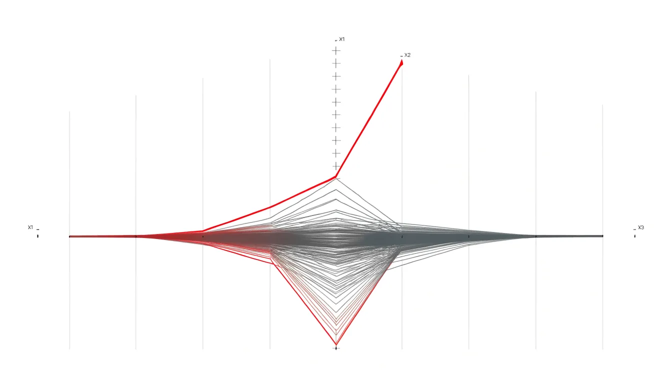
Multivariate anomalies require closer attention, since no single coordinate looks remarkable on its own. Here the clue lies in unusual combinations of positions across several axes: a line that threads through the low end of one variable, the high end of the next, and an intermediate band on a third may never touch an extreme value yet still trace a path no other observation follows. These lines weave against the grain of the dominant bundles, crossing them at steep angles and occupying empty regions of the plot between axes. By scanning for polylines that leave the main flow and remain isolated across multiple dimensions, analysts can flag records whose joint attribute configuration is rare or suspicious, even though each individual value falls within a normal range.
Parallel Coordinates Plot
Datasets with thousands of observations quickly produce a mat of overlapping strokes in which individual trajectories, trends, and outliers dissolve into undifferentiated ink. Overlap is not random noise but a direct function of dataset size and attribute similarity: records that share values on several axes trace nearly identical paths, and those paths pile up in the same screen regions.
Several techniques reduce the number of marks the eye must separate:
- Downsampling draws a representative subset of lines, either uniformly at random or through stratified or importance-based sampling that preserves coverage of extreme and mid-range observations. The tradeoff is that rare patterns may be dropped, so sampling schemes must match the analytical question.
- Line density aggregation summarizes where lines concentrate rather than showing each line. The plane between adjacent axes is divided into bins, each bin receives a count of lines passing through it, and the counts are rendered as a color or opacity gradient, converting a tangle of strokes into a smooth density field that highlights dominant flows and exposes sparse regions.
- Curve bundling addresses overlap geometrically. Nearby polylines are routed together into shared bundles, much as hierarchical edge bundling merges related connections, so that a thick cord represents many similar records while individual lines peel away where their values diverge. Bundling keeps visual complexity proportional to the number of distinct patterns rather than the number of raw records.
In practice these techniques combine well: aggregation for the global structure, bundling for grouped trajectories, and selective downsampling plus interactive highlighting for detailed inspection of individual records on demand.
Parallel Coordinates Plot
Strategic use of alpha transparency also solves much of the overplotting problem. By lowering the opacity of each line, regions where many observations share similar value patterns accumulate into darker, denser bands, while sparse areas remain faint. This turns overplotting into a visual asset, drawing the eye to the clustering structure of the data where dense corridors between axes indicate common trajectories and divergent paths remain visible.
Color adds a second, independent channel of information on top of position:
- Categorical color palettes assign distinct hues to classes of a target variable, letting viewers separate groups and observe where their profile lines cross or converge.
- Sequential gradients suit continuous target variables, with a light-to-dark ramp encoding magnitude along each polyline.
Class membership or target intensity remains readable even in crowded regions because hue and luminance distinguish lines that would otherwise blur together.
Combining transparency with color requires calibration. Alpha values should be low enough to prevent saturation but high enough that solitary lines remain perceptible. Color ramps should preserve contrast when applied at partial opacity, and legends should clarify what each hue or shade represents.
Parallel Coordinates Plot
The ordering of the axes directly influences the visual patterns that emerge in a parallel coordinates plot. Relationships between variables are most easily detected when their axes are adjacent, because the line segments between them are short and direct. When two correlated variables are placed far apart, their relationship is obscured by the intervening axes, making it difficult to perceive trends such as clustering or inverse correlations.
To uncover hidden patterns, analysts reorder axes dynamically. A common strategy is to place variables with known or suspected relationships next to each other, though this requires prior knowledge. Automated algorithms offer a more systematic approach by evaluating all possible permutations or using heuristics to find an order that maximizes the visibility of correlations. These algorithms often measure the clutter or overlap of lines between adjacent axes and seek to minimize it, or use similarity metrics such as correlation coefficients or mutual information to group related variables together.
Interactive tools allow users to manually swap axes and immediately see the effect on the plot, sometimes animating the transition to help users track changes. By strategically reordering axes, analysts can reveal non-adjacent correlations that were previously hidden, such as a strong negative correlation between two variables initially placed at opposite ends of the plot.
Parallel Coordinates Plot
Interactive brushing turns a parallel coordinates plot from a static overview into a live analytical instrument. A user clicks and drags along a segment of a chosen axis, and the system selects every line whose value falls within that vertical interval. The selected lines are highlighted while the remaining lines are dimmed or removed, making the filtered subset stand out against the broader population.
The power of the technique comes from combining brushes across multiple axes. Dragging a range on one axis narrows the visible records to those matching that criterion, and adding a second brush on another axis further constrains the selection to records satisfying both conditions simultaneously. Because each added constraint intersects with the previous ones, users can iteratively sculpt a query that targets a complex sub-population, such as observations with high values on one dimension, moderate values on a second, and low values on a third. The plot updates as each brush is drawn, giving immediate visual feedback on how many lines survive and where they fall on the remaining axes.
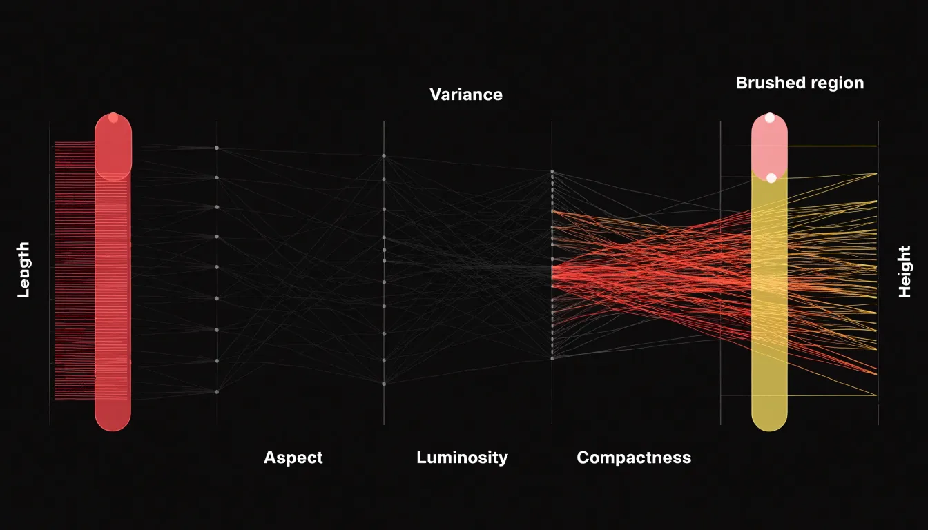
This dynamic filtering supports real-time exploration of populations that would be difficult to isolate through numeric queries alone. Analysts can test hypotheses about which variable combinations define a group, observe how a selected cluster behaves across dimensions outside the filter, and adjust or remove brushes to recover context while keeping the full dataset in view.
Parallel Coordinates Plot
Cluster analysis provides a statistical route to grouping similar data points in a parallel coordinates plot. Algorithms such as k-means, hierarchical clustering, or density-based methods operate on the multivariate records, assigning each observation to a cluster based on the similarity of its values across the axes. Once these cluster assignments exist, they can be used as class labels and mapped to color, so that every line belonging to a given group shares a hue. Line bundles then visually separate into distinct, color-coded functional groups, and a viewer can follow the shape of each bundle across the full set of axes without tracing individual records.
Class labels that already exist in the data—such as customer tier, machine state, or experimental condition—serve the same segmenting role. Coloring lines by label transforms the plot into a comparison instrument where bundles diverge on some axes and converge on others.
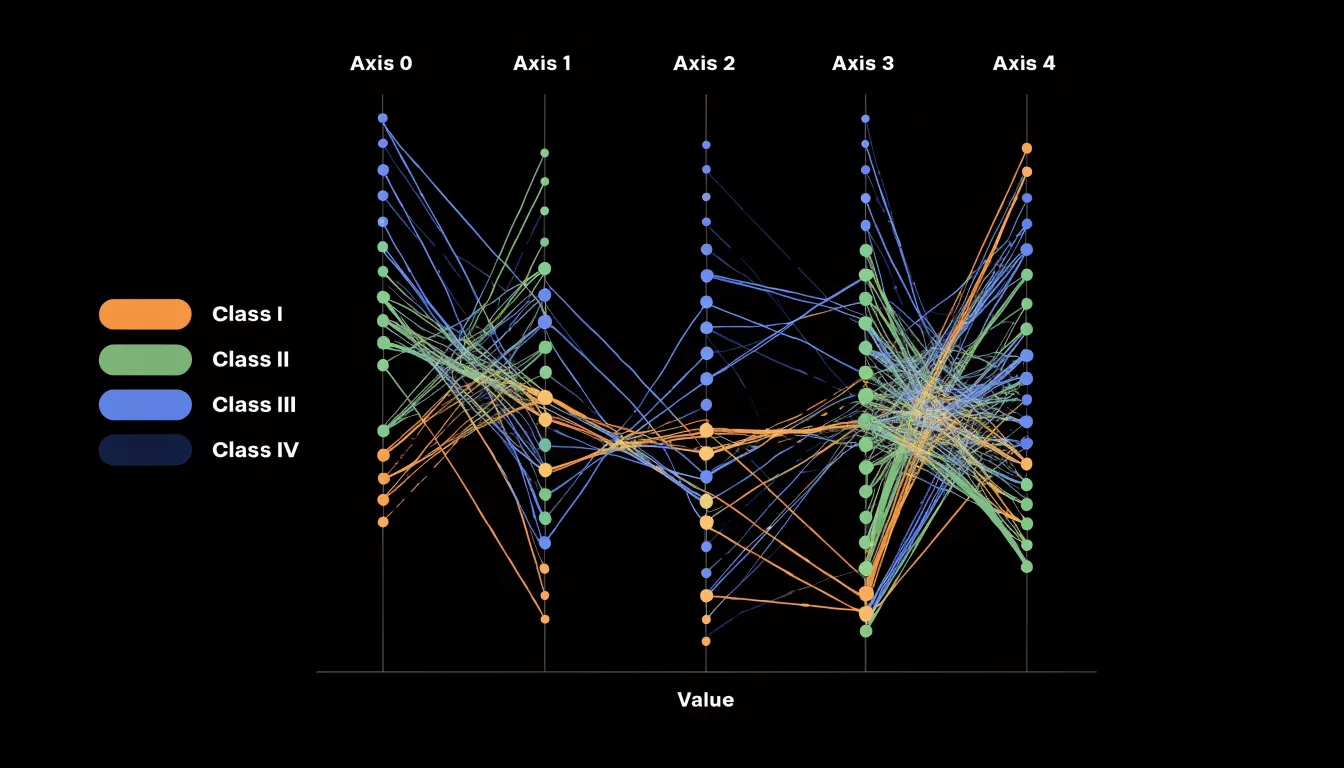
Comparing the profile shapes of the bundles is where domain insight emerges. A group whose lines rise steeply between two adjacent axes followed by a plateau tells a different story from a group that descends gradually across the whole range. These characteristic shapes often correspond to recognizable personas, behavioral types, or operating regimes within the domain, giving analysts a vocabulary for describing segments that raw numbers alone do not supply. Interactive brushing can then isolate a bundle to confirm which axes drive the separation and which are shared across groups.
Parallel Coordinates Plot
Parallel coordinates plots let business decision-makers evaluate many attributes at once without collapsing them into a single score.
- Customer segmentation: A marketing team can plot customers or segments across axes for age, lifetime value, purchase frequency, average order size, and churn probability. A cluster of lines that stays tightly bundled across every axis points to a stable high-value group worth a dedicated retention campaign, while lines that diverge sharply between purchase frequency and lifetime value flag customers whose future spending is uncertain.
- Product feature trade-offs: When evaluating configurations, each design can be drawn across axes for cost, weight, battery life, manufacturing complexity, and customer satisfaction rating. Reviewers can trace individual lines to see which designs stay competitive across all requirements and which excel on one dimension at the expense of others, helping product and sales teams communicate options to clients and narrow candidates before deeper testing.
- Financial risk profiles: A lender or treasury group can plot loan applicants or portfolio holdings across axes for credit score, debt-to-income ratio, exposure, collateral value, and default history. Lines that bend sharply at a given axis reveal where risk concentrates, supporting faster triage.
Across these cases, marketing teams can compare campaign targeting rules, sales teams can align offers with customer constraints, and finance teams can adjust terms before losses accumulate. Keeping the reasoning visible makes it easier to justify decisions in cross-functional meetings and revise assumptions as new data arrives.
Parallel Coordinates Plot
Scientific and environmental monitoring frequently involves observations with dozens of sensor readings, climate model parameters, or genomic variations.
- Environmental monitoring: Sensor networks record temperature, humidity, particulate matter, wind speed, and other indicators at high frequency. Plotting these readings in parallel coordinates helps analysts identify anomalous events, such as a pollution spike coinciding with specific wind conditions and humidity levels. In one case study tracking urban air quality, parallel coordinates revealed that high particulate matter concentrations were consistently associated with low wind speeds and specific temperature inversions, guiding targeted interventions.
- Climate model parameters: Researchers use parallel coordinates to compare model runs against observational data, highlighting parameter combinations that lead to realistic simulations. In one study, tracking temperature, precipitation, and cloud cover simultaneously helped isolate a set of parameters that reduced uncertainty in regional climate projections.
- Genomic data variations: By plotting gene expression levels and single nucleotide polymorphisms across thousands of genomic features, scientists detect patterns associated with disease subtypes or environmental responses. A case study examining gene expression across multiple environmental conditions uncovered coordinated changes in gene clusters that traditional pairwise analyses missed.
Parallel Coordinates Plot
Parallel coordinates plots serve machine learning engineers as a visual dashboard for comparing many experimental runs side by side.
- Hyperparameter tuning: Each vertical axis represents one hyperparameter—such as learning rate, batch size, dropout rate, or number of hidden layers—while each polyline traces a single trial. When dozens or hundreds of trials are overlaid, clusters of lines converging on particular axis regions reveal parameter ranges worth exploring further, while scattered, tangled segments flag settings that produce erratic behavior. This makes the plot a practical companion to grid search or Bayesian optimization.
- Model performance metrics: Separate axes can hold accuracy, precision, recall, F1 score, latency, and memory footprint, showing the full profile of one model run in a single line. Engineers can identify runs that balance competing metrics and spot trade-offs between speed and accuracy. In classification problems, the plot helps visualize trade-offs between false positive and false negative rates across different decision thresholds or architectures.
- Feature importance: When axes are assigned to individual features or importance scores, lines that stay high on a given feature axis across strong-performing runs suggest that feature carries consistent predictive weight, while features with widely varying values across good runs may be less critical or more context-dependent.
Parallel Coordinates Plot
Design mistakes in parallel coordinates plots often begin with axis scaling. When each vertical axis uses its own raw measurement units, a variable measured in thousands sits beside one measured in single digits, and the resulting line slopes reflect unit differences rather than data patterns. Viewers read steep crossings as dramatic change and flat segments as stability, even when the underlying variation is identical. Normalizing every axis to a common range, such as zero to one, or clearly labeling units and chosen bounds, prevents visual artifacts that suggest relationships where none exist.
Common pitfalls and their remedies include:
- Static displays: Without interaction—brushing a range, highlighting a subset, reordering axes, or hovering to inspect a line—dense regions collapse into a solid band and outliers disappear into the mass. Offering linked highlighting and axis reordering lets viewers follow a single observation and test how the structure changes.
- Unmanaged line density: With hundreds of records, overplotting hides patterns and creates false impressions of uniformity. Transparency, aggregation, density shading, or sampling strategies preserve the sense of how many observations share a trajectory while keeping individual paths visible.
- Poor color choices: Rainbow palettes imply ordering that does not exist, low-contrast hues vanish against white backgrounds, and colors applied without meaning invite misreading. Use restrained, purposeful palettes tied to a clear variable with sufficient contrast against the background.
Parallel Coordinates Plot
Building an interactive parallel coordinates plot begins with choosing a tool that matches the team’s technical skills and delivery environment:
- D3.js offers the most granular control, letting developers draw each axis, line path, and brush interaction from scratch, which suits bespoke dashboards where visual identity and custom interaction patterns matter.
- Plotly provides a faster route for Python and JavaScript users, with a high-level parallel coordinates trace that supports brushing, axis reordering, and hover tooltips out of the box.
- Python’s data ecosystem supports rapid prototyping: pandas handles data wrangling, scikit-learn offers utilities for scaling dimensions before plotting, and libraries such as Plotly Express and Altair let teams iterate quickly before committing to a production build.
- Tableau serves organizations that favor a governed, drag-and-drop environment, where parallel coordinates views can be assembled through calculated fields and dashboard actions that filter companion charts on the same sheet.
When embedding these charts into executive dashboards, limit the number of axes to the handful of dimensions that drive the decision at hand, normalize each axis to a consistent scale, and order axes to tell a coherent story rather than following the raw column order of the dataset. Use a restrained color palette to encode a single categorical dimension such as segment or region, and provide brushing controls that update companion charts so executives can move from an aggregate overview to a specific cohort. Finally, pair the plot with a short annotation or caption that names the primary multivariate pattern worth noticing.
Frequently Asked Questions
What is a parallel coordinates plot used for?
A parallel coordinates plot arranges each variable as its own vertical axis side by side, and each record becomes a polyline crossing every axis at its value. It lets an analyst follow one data instance across many attributes and see correlations, clusters, and outliers in a single view.
How do you read correlations on a parallel coordinates plot?
Between adjacent axes, positive relationships appear as lines running roughly parallel or converging into a tight band, while inverse relationships appear as lines crossing in a dense braid. Scanning the chart from left to right and treating each pair of adjacent axes as a small scatter of slopes helps read these patterns.
How do you spot outliers in a parallel coordinates plot?
A single-variable extreme value often appears as a spike or deep notch where a line stretches away from the bundle at one axis and returns toward the central mass on neighboring axes. Multivariate anomalies may never touch an extreme value but show unusual combinations across several axes, weaving against the dominant bundles and occupying empty regions of the plot.
How do you handle too many lines in a parallel coordinates plot?
Techniques include downsampling, line density aggregation, curve bundling, and alpha transparency. These reduce the number of marks the eye must separate or turn overplotting into a visual signal of where many observations share similar trajectories.
Does axis order matter in a parallel coordinates plot?
Yes. Relationships between variables are most easily detected when their axes are adjacent, because the line segments between them are short and direct. Analysts can reorder axes dynamically, and automated algorithms can evaluate permutations or use heuristics to group related variables and reduce clutter.
What does brushing do in a parallel coordinates plot?
Brushing lets a user click and drag along a segment of an axis to select every line whose value falls within that vertical interval, highlighting the selected lines while dimming or removing the rest. Combining brushes across multiple axes further narrows the selection to records satisfying all conditions simultaneously.
Tony Astor
Tony writes about data visualization and the tools people use to build charts and dashboards. More about Data Illustrator