Mosaic Plot: Visualizing Categorical Data Proportions
 By Tony Astor ·

Mosaic Plot
A mosaic plot displays the relationship between two or more categorical variables by dividing a fixed-area rectangle into tiles whose widths reflect each category’s marginal proportion and whose heights reflect conditional proportions within that category. Each tile’s area therefore equals its joint proportion, making associations, independence, and rare combinations visible at a glance.
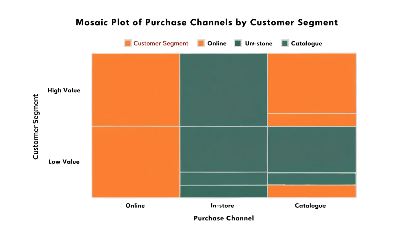
Table of Contents
Mosaic Plot
A mosaic plot offers a compact way to compare proportions across two categorical variables at once. The plotting area is divided first along one axis according to the marginal proportions of the first categorical variable, so the width of each column reflects how much of the total sample falls into that category. Each column is then split vertically according to the conditional proportions of the second variable within that column, so the height of each segment reflects the share of that group belonging to the second category. The result is a grid of rectangles whose widths and heights each carry information, and whose areas therefore represent the joint distribution probabilities directly.
Because the overall plot always has a fixed total area, a large rectangle signals a common combination and a small sliver signals a rare one, all within the same visual frame. Comparing the vertical splits from one column to the next shows how the distribution of the second variable shifts as the first variable changes. If the splits are aligned across columns, the two variables behave independently; if the split points rise or fall noticeably between columns, an association is present. This makes conditional comparisons immediate, since the eye can track a single horizontal boundary across adjacent columns and see whether the proportions hold steady or drift.
Mosaic plots are especially useful when at least one variable has several categories and a simple two-way table would be dense to read. They also scale to more than two variables through recursive splitting, though the two-variable form remains the most common. With careful ordering of categories, graduated shading, or labels, a mosaic plot turns a table of counts into a picture where differences in proportion and joint probability stand out clearly.
Two-Way Tables
A two-way table organizes data by two categorical variables simultaneously, producing a grid of frequency counts known as a contingency table. Each row represents a category of the first variable, each column a category of the second, and each interior cell holds the count of observations falling into that particular combination. While this structure is compact and precise, reading patterns across dozens of cells requires careful scanning and mental arithmetic.
The mosaic plot shows the same information by mapping frequency to geometry. The full plotting rectangle represents the entire dataset, and its area is partitioned so that each cell of the contingency table receives a sub-rectangle whose area is proportional to its count. A cell with twice the count of another occupies twice the visual space, whether through greater width, greater height, or both. This proportional mapping allows the eye to compare categories directly, spot unusually large or sparse combinations, and perceive the overall structure of association between the two variables without consulting the numbers themselves. Color or shading can be layered on top to highlight deviations from expected counts, but the underlying spatial geometry already communicates the core information of the original table.
Tile Area
To read proportions accurately in a mosaic plot, you need to understand what each dimension of a tile contributes. Because a tile’s area is the product of its width (the marginal proportion of the column variable) and its height (the conditional proportion within that column), multiplying the two recovers the joint proportion of the total observations.
A practical example clarifies the decoding. Suppose a column occupies 40 percent of the plot’s width, and a tile inside it reaches 50 percent of the column’s height. The tile’s area is 0.40 times 0.50, giving 0.20, or 20 percent of all observations. Reading the height alone would mislead you into reporting 50 percent, which is the conditional share within that column rather than the overall share. Conversely, two tiles with equal areas represent equal counts or proportions, even if one is tall and narrow and the other short and wide.
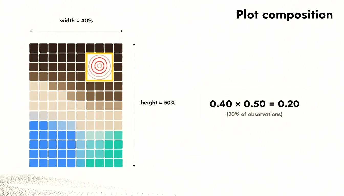
Because both dimensions matter, the eye can be deceived by shape. A tall, thin tile and a short, wide tile may cover similar areas while looking very different. To decode exact percentages, multiply the relative width by the relative height, or read the axis scales carefully. Checking that column widths sum to the full width and that heights within each column sum to that column’s height provides a useful consistency check.
Group Comparisons
Once the overall structure of a mosaic plot is clear, the analyst turns to how sub-groups behave relative to one another and to the whole. Moving the eye across categories reveals where the balance of representation shifts. A segment containing far more of one sub-group than its overall frequency would suggest stands out immediately, drawing attention to a disproportionate representation that might remain buried in a table of counts.
Skewness within categories emerges naturally from this comparison. Some segments may be dominated by a single sub-group, producing a lopsided internal split, while others are split more evenly. Reading across the plot shows whether that lopsidedness is consistent or changes from segment to segment. When the relative heights or widths of subdivided tiles shift markedly across segments, the plot signals a conditional probability shift worth investigating further.
These comparisons work best when the analyst scans systematically, moving from the largest segments down to the smaller ones and noting where the internal composition diverges from the baseline. Disproportionate sub-group representation often surfaces at the margins, where a minor category is almost entirely composed of one sub-group. Such findings invite follow-up questions about the data-generating process, sampling, or genuine structural differences between groups.
Independence and Association
Judging whether two categorical variables influence each other rests on a simple benchmark: statistical independence. If the row and column variables are unrelated, the proportion of cases falling into any row category should stay roughly constant across every column category. Under independence, the heights of corresponding tiles line up across column breaks, producing a flat, level profile from left to right. When association is present, those heights rise and fall across columns, and the eye picks up the unevenness without calculation.
Pearson residuals put numbers behind that visual read. Each cell’s residual compares the observed count with the count expected under independence, scaled by the square root of the expected count. A residual near zero signals a cell that behaves as independence predicts, and the overall mosaic stays level. Large positive residuals mark cells that occur more often than expected, while large negative residuals mark cells that occur less often. Because the residuals are standardized, cells with values beyond roughly two or three deserve attention, and a pattern of alternating large positive and large negative residuals across a row or column is the numerical fingerprint of association.
Reading the plot this way combines the global and the local picture. The overall contour of tile heights answers whether the variables are associated at all, and the size of individual tiles relative to their column totals shows which categories drive the departure. Uneven tile heights that persist across many columns indicate a systematic relationship, while a single jagged column often reflects a small sample or an outlier category. Checking these features in concert turns the mosaic plot into a practical screen for association before any formal chi-square test is run.
Color and Shading
Color and shading transform a mosaic plot from a display of cell proportions into a diagnostic tool for statistical significance. The standard approach ties a color scheme to standardized residuals, mapping positive deviations onto blue tones and negative deviations onto red tones. This lets viewers read the direction and magnitude of departures from independence at a glance, without consulting a separate table of test statistics.
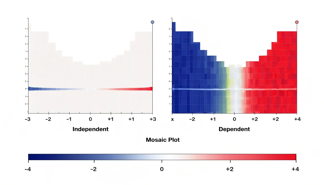
The shading typically follows a diverging palette centered on a neutral color at zero residual. Small residuals receive pale or muted tones, signaling little departure from independence. As residuals grow larger in absolute value, the color deepens toward saturated blue or red. Many implementations anchor the color scale to conventional significance thresholds, so that a residual corresponding to a p-value around 0.05 already shows visible color, and cells exceeding stricter thresholds such as 0.01 or 0.001 appear in the deepest shades. This calibration ties visual intensity directly to statistical evidence, helping distinguish meaningful departures from sampling noise.
Across a plot of many cells, shading reveals patterns that raw area alone can obscure. Clusters of similarly colored cells point to categories whose associations drive the overall test result, while a mosaic dominated by pale tones suggests the independence model fits reasonably well. Patterned shading also draws attention to outliers and interactions between variables that might otherwise be buried in a dense layout.
Multidimensional Data
When a contingency table grows beyond two categorical variables, a mosaic plot’s recursive partitioning scheme extends naturally to handle the added dimensions. To introduce a third variable, the plot divides the total area by the levels of the first variable, subdivides each segment by the second variable, and then subdivides each second-level cell by the levels of the third. Every nested split preserves the proportional-area convention, creating a hierarchy of rectangles whose sizes can be read at any depth to trace how the joint distribution shifts as additional variables enter the model.
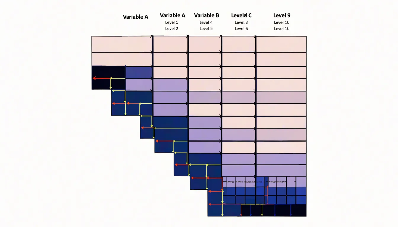
Extending the logic to a fourth variable adds another layer of subdivision inside each third-level cell. The dimensions of the plot remain fixed, and the algorithm alternates splitting directions so that successive variables are laid out along perpendicular axes. This alternation keeps sub-cells legible and gives the eye a predictable rhythm to follow. Conditioning becomes explicit: each tile is understood relative to its parent segment, so conditional independence and interaction can be assessed at every branch of the tree.
The practical challenge is scale. Each additional variable multiplies the number of terminal tiles, and small cell counts can collapse into slivers that are hard to distinguish. Analysts manage label density, level ordering, and shading to keep the structure readable. Ordering levels by frequency or similarity and grouping rare categories into residual buckets preserves interpretability while retaining the multivariate picture that three- and four-way contingency tables demand.
Survey Analysis
Survey analysis in market research often mixes demographic variables—such as age bracket, income level, region, and product category—with behavioral outcomes like purchase frequency or brand loyalty. Splitting a mosaic plot first along a demographic variable and then by purchasing behavior shows whether buying habits shift across consumer groups. A segment dominated by frequent buyers appears as a row of tall, adjacent rectangles, while a group with scattered preferences shows a more fragmented pattern. This makes mosaic plots useful during exploratory analysis to generate hypotheses about which demographic factors matter and where deeper statistical testing should focus.
The visual encoding also helps communicate findings to stakeholders who may not be comfortable reading cross-tabulations. Instead of scanning dozens of percentage cells, a marketing team can point to a specific region of the plot and discuss why younger urban respondents cluster around one product tier while older suburban respondents spread across several. In practice, mosaic plots work best alongside conventional measures such as chi-square tests, serving as a first pass before formal modeling. When survey datasets span many categorical dimensions, careful ordering of the split variables and sensible grouping of categories keep insights actionable for segmentation and targeting decisions.
Demographics
Demographic analysis focuses on how population traits cluster and intersect rather than on a single variable in isolation. Applied to census data, a mosaic plot shows how age groups distribute across income brackets, or how geographic regions differ in household composition.
The same logic applies to user profile data. A product team might examine how subscription tiers break down by age range, or how device type varies across geographic markets. Imbalances become immediately visible: a wide column paired with a thin segment signals a large group with a small share in a secondary category, while a narrow column with a tall segment points to a smaller group heavily concentrated in one trait. Adjacent columns invite direct inspection of how composition shifts from one region or cohort to the next, highlighting which intersections deserve closer modeling and which categories account for the bulk of variation in the population.
Mosaic Plot vs Bar Chart
When displaying the relationship between two categorical variables, choosing between a stacked bar chart and a mosaic plot hinges on which aspect of the data deserves visual emphasis.
In a stacked bar chart, every bar has the same width, and internal segments show the distribution across the second variable. The fixed width gives each primary category the same visual weight, making it straightforward to compare internal compositions across groups. This works best when the primary categories are roughly equal in size, or when their relative sizes are not the central focus.
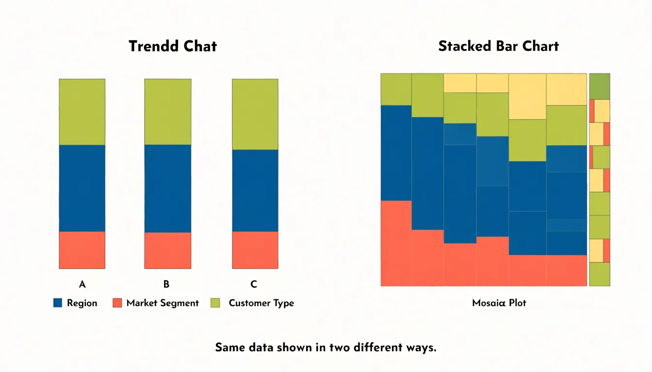
A mosaic plot makes column width proportional to the primary category’s total count or share, revealing both marginal totals and internal composition at once. Small groups visibly shrink, and large groups dominate the plot area. This variable-width encoding is useful when the overall size of each category matters as much as its internal structure.
The trade-off is legibility. Equal-width bars support precise comparison of proportions because the reference frame stays constant across groups, while variable-width segments in a mosaic plot can become narrow and hard to read when a category is small or heavily subdivided. For audiences unfamiliar with the format, varying widths may also require extra interpretation. If the task is comparing compositions across groups of similar scale, a stacked bar chart keeps proportions clear; if the task is understanding how group size and internal distribution interact across the dataset, a mosaic plot communicates that structure more faithfully.
Mosaic Plot vs Treemap
Mosaic plots and treemaps both divide a rectangle into smaller regions, making them easy to confuse and frequently misapplied. However, their underlying structures answer different questions.
- Treemaps organize data hierarchically. Each rectangle represents a node in a tree, and nested rectangles show part-to-whole relationships across levels, with area proportional to a single quantitative measure such as revenue or file size. The layout algorithm packs sibling rectangles together by size. Treemaps suit questions about composition and relative magnitude within hierarchies, such as which product lines dominate a portfolio.
- Mosaic plots begin with a two-way or multi-way contingency table, splitting the plot horizontally by one categorical variable and subdividing the resulting bands proportionally by subsequent variables. Widths and heights encode conditional proportions rather than a continuous magnitude, making patterns of association and independence visible through deviations from an even grid. Mosaic plots suit questions about relationships between categorical variables, such as whether customer segments differ in their purchase channel mix or whether outcomes vary across treatment groups.
A common charting mistake is building a mosaic plot for non-categorical numeric data or hierarchy-only questions, where the subdivision logic adds visual complexity without analytic payoff. Equally common is using a treemap to compare category combinations, which obscures the proportional structure the mosaic plot is designed to reveal.
Common Reading Pitfalls
Misreading tile geometry is a frequent source of error in mosaic plots:
- Confusing tile width with absolute sample size: Column width represents a category’s share of the total sample, not the raw count. A wide column may reflect a large share of a small overall sample, while a narrow column in a large dataset could contain many more observations in absolute terms. Focusing on width alone can overestimate the importance of a category that is proportionally large but numerically modest.
- Comparing heights without considering width: Because tile height shows a conditional proportion within a column, a tall tile in a narrow column may represent fewer cases than a shorter tile in a wide column. Ignoring this interplay leads to incorrect conclusions about which combinations are most common.
- Over-interpreting low-count cells: When a cell contains very few observations, its tile area can be disproportionately influenced by rounding or overall plot scaling, and its proportions may fluctuate widely with small changes in the data. Readers should avoid drawing strong inferences from tiny tiles.
To avoid these pitfalls, compare areas rather than single dimensions, and supplement the visual with a table of frequencies when precise counts matter.
Design Best Practices
Thoughtful labeling, color selection, and layout refinement keep a mosaic plot readable:
- Labels and annotations: When category names are long or numerous, rotate horizontal axis labels to a 45-degree angle to prevent overlapping while maintaining readability. Keep vertical axis labels horizontal to avoid neck strain. Include a clear title and subtitle stating the variables and their order, and consider adding percentage annotations inside cells to reduce reliance on the axes.
- Color palettes: Choose colorblind-safe scales such as viridis or ColorBrewer’s qualitative palettes, which remain distinguishable for viewers with deuteranopia or protanopia, and avoid red-green contrasts. Use consistent color mapping across panels in faceted plots, and reserve high saturation for highlighting key categories while muting others. For sequential data, use a perceptually uniform gradient so shading differences accurately reflect magnitude differences.
- Whitespace and borders: Increase outer margins so labels are not cut off, and adjust spacing between cells to create a subtle grid that aids comparison. Remove unnecessary gridlines and background fills, keep cell borders thin and neutral, and ensure text inside cells has sufficient contrast against the fill color.
Building Mosaic Plots
Building a mosaic plot starts with preparing categorical data as a contingency table or a data frame with two or more categorical columns.
- R (
vcdpackage): Create a contingency table withtable(), then pass it tomosaic(). Theshadingargument colors tiles by the standardized residuals of a chi-squared test, whilegpandlabeling_argscontrol colors, borders, and labels. Thesplitanddirectionarguments determine which variable defines the columns and which defines the rows. Runningassoc()beforehand helps inspect the residual structure that the shading will display. - Python (
statsmodels): Themosaic()function in the graphics module accepts a contingency table—typically built withpandas.crosstab()—along with the index of the variable to place on the x-axis. It returns amatplotlibfigure and axes object, allowing standardmatplotlibcustomization for colors, labels, annotations, and figure size. - Tableau: Because Tableau lacks a built-in mosaic plot, you construct one manually from a stacked bar chart. Place the first categorical dimension on columns, the second on rows, and the measure on bar length. Set the view to percentage of total, adjust the mark size, and configure the stacked bars to fill the width. Dual-axis and axis synchronization tricks align segment widths across categories, enabling interactive filtering and tooltips for dashboards.
Interactive Dashboards
Rendering a mosaic plot in an interactive library such as Plotly or D3.js turns each rectangle into an event-bearing element. Hovering over a tile can raise a tooltip showing the observed count, expected count under independence, standardized residual, row and column percentages, and the confidence interval for the proportion. This immediate feedback removes the need to cross-reference a printed table and helps viewers judge whether an association is substantive or an artifact of small cell sizes.
Drill-down capabilities extend the analysis across levels of detail. Clicking a column segment in a two-variable mosaic can re-render the display conditioned on that level, revealing how associations shift within a subgroup. Breadcrumb navigation and bidirectional linking let users step back to the overview without losing context. With linked selection across coordinated views, highlighting a tile in the mosaic can also filter a companion bar chart or table.
Real-time filtering completes the workflow. Controls for category subsets, date ranges, or minimum cell counts feed directly into the data pipeline so the layout updates instantly, while transition animations help viewers track how tiles grow, shrink, or reorder between states.
Frequently Asked Questions
What is a mosaic plot used for?
A mosaic plot is used to compare proportions across two categorical variables at once, with tile areas representing joint distribution probabilities. It is especially useful when at least one variable has several categories and a simple two-way table would be dense to read.
How do you calculate what a tile represents in a mosaic plot?
A tile’s area is the product of its width, the marginal proportion of the column variable, and its height, the conditional proportion within that column. For example, a column occupying 40 percent of the plot width with a tile at 50 percent of the column height represents 0.40 times 0.50, or 20 percent of all observations.
How can you tell if two categorical variables are independent in a mosaic plot?
If the splits are aligned across columns and the profile stays level, the two variables behave independently; if split points rise or fall noticeably between columns, an association is present. Pearson residuals near zero signal cells behaving as independence predicts, while values beyond roughly two or three deserve attention.
What do the colors or shading mean in a mosaic plot?
The standard approach maps positive standardized residuals to blue tones and negative residuals to red tones, centered on a neutral color at zero residual. Small residuals get pale or muted tones, while larger residuals deepen toward saturated blue or red, with many implementations tying color to significance thresholds such as 0.05, 0.01, or 0.001.
When should you use a mosaic plot instead of a stacked bar chart?
A stacked bar chart uses equal-width bars, making it straightforward to compare internal compositions across groups. A mosaic plot makes column width proportional to the primary category’s total count or share, revealing both marginal totals and internal composition at once, though variable-width segments can become narrow and hard to read.
What are common mistakes when reading a mosaic plot?
Common mistakes include confusing tile width with absolute sample size, comparing heights without considering width, and over-interpreting low-count cells. To avoid these pitfalls, compare areas rather than single dimensions and supplement the visual with a table of frequencies when precise counts matter.
Tony Astor
Tony writes about data visualization and the tools people use to build charts and dashboards. More about Data Illustrator