Misleading Charts: Common Tricks and How to Spot Them
 By Tony Astor ·

Misleading Charts
Misleading charts distort data through truncated or inverted axes, omitted baselines, cherry-picked timeframes, cumulative totals, unlinked dual axes, improper symbol scaling, 3D pie charts, unequal category sizes, loaded colors, raw population counts, selective smoothing, and misplaced trend lines. Each technique exaggerates small differences or hides declines, so readers should verify axis scales, baselines, timeframes, denominators, and printed values before trusting a chart’s visual impression.
Table of Contents
- Truncated Y Axis
- Inverted Scale
- Omitted Baseline
- Cherry-Picked Timeframes
- Cumulative Growth Charts
- Unlinked Dual Axes
- Improper Symbol Scaling
- Oversized Pie Charts
- Unequal Category Sizes
- Misleading Color Choices
- Ignoring Population Sizes
- Selective Data Smoothing
- Misplaced Trend Lines
- Essential Checklist
Truncated Y Axis
A truncated y-axis exaggerates change by starting the vertical scale at a value higher than zero, compressing the visible plotting area into a narrow band. When the axis is cut off this way, a fluctuation of a few percentage points can stretch across most of the chart’s height, giving the impression of a dramatic surge or collapse. Readers absorb the shape of the line or the height of the bars long before they examine the tick marks, so the truncated scale does its work quietly.
A typical real-world case involves stock prices or sales figures. A company’s share price moving from 102 to 108 dollars looks like a dramatic spike when the axis runs from 100 to 110, even though the change is under six percent. The same data plotted from zero appears as a nearly flat line. Similar distortions appear in polling charts, where approval ratings drifting from 48 to 52 percent can be rendered as a steep climb by setting the axis bounds to 45 and 55. Budget charts and performance dashboards use the same trick, cropping the scale to amplify small differences between competing options.
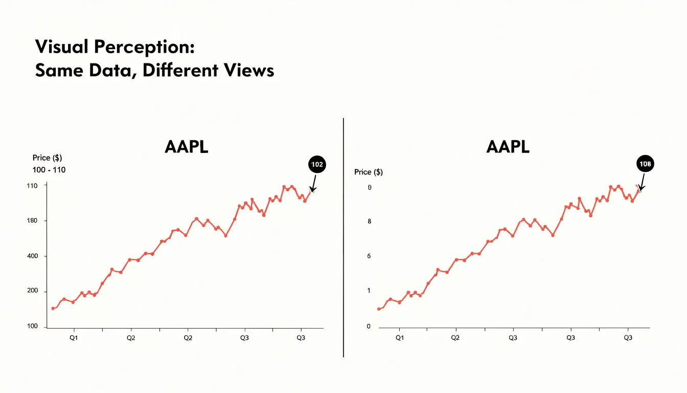
Spotting a manipulated axis takes a few deliberate habits:
- Locate the bottom of the vertical scale and check whether it starts at zero.
- Note the distance between tick marks and confirm the intervals are consistent.
- Compare the visual change to the actual numeric change by reading the labeled values at the start and end of the plotted line.
- Calculate the percentage change mentally against the axis range to see whether the bounds are informing or persuading.
Inverted Scale
An inverted scale occurs when the vertical axis of a chart is flipped so that higher numerical values sit at the bottom and lower values sit at the top. To a casual reader, the chart still looks like a standard graph, with a line climbing upward or a bar rising from a baseline. The eye follows that upward motion and reads it as growth, because decades of exposure to ordinary charts have trained viewers to associate up with more. When the axis is reversed, however, up means less. A line that appears to surge toward the top of the frame may actually be tracking a steady decline, while a bar that seems to shrink is really expanding.
Because only the axis labels reveal the trick, inverted scales have appeared in major news outlets—sometimes by accident and sometimes through deliberate framing choices. A well-known example is the Fox News broadcast graphic that showed unemployment data with a flipped vertical axis, making a falling unemployment rate appear as a rising trend. A similar controversy surrounded an inverted-axis chart circulated during discussions of firearms statistics, where the visual slope contradicted the actual direction of the numbers.
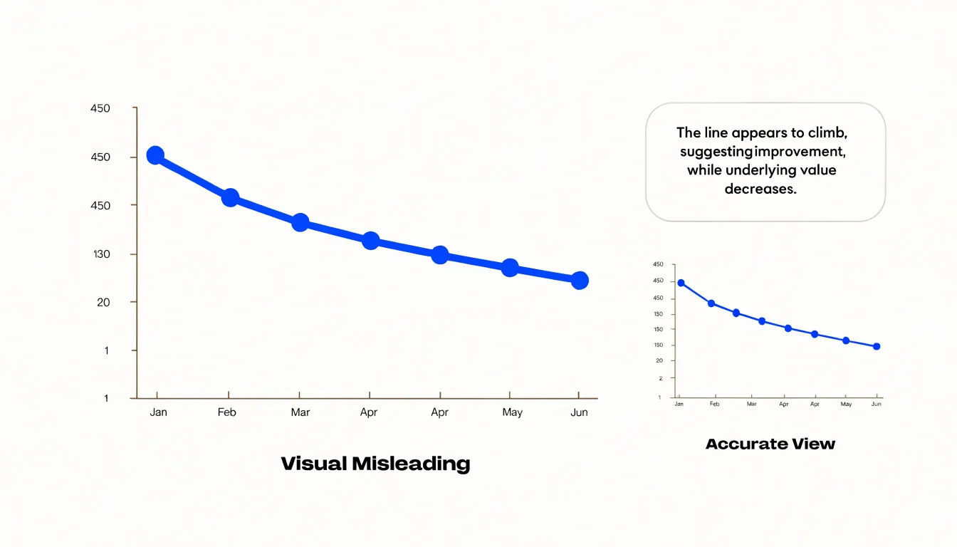
Once an inverted graphic spreads through social media, the impression it creates can outlast any correction, as audiences remember the shape of the line far longer than an explanatory note. For anyone building charts, the safeguard is straightforward: keep the conventional orientation unless there is a compelling reason, label the axis prominently, and review the final graphic with a fresh eye before publication.
Omitted Baseline
While a non-zero baseline in a line chart is sometimes acceptable for showing trends over time (if clearly labeled), omitting the zero baseline in a bar chart breaks its core encoding. Because the human eye compares the full lengths of bars from the baseline, each bar’s height must represent the entire magnitude of the value. When the vertical axis starts above zero, the bar represents only the portion above the chosen starting point, distorting the visual ratio between categories.
For example, if two values are 100 and 110, a bar chart starting at zero shows the second bar as 10% taller than the first. If the axis starts at 95, the first bar extends 5 units above the baseline while the second extends 15 units, making the second bar appear three times as tall.
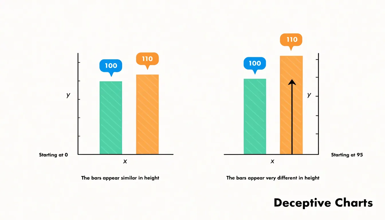
To preserve proportional accuracy, bar charts comparing magnitudes should always start at zero. If a non-zero baseline is unavoidable in other chart types, designers should provide clear indicators of the truncated axis or consider alternative representations that show differences directly.
Cherry-Picked Timeframes
By carefully selecting the start and end points of a graph, a chart maker can hide a broader trend and create a false impression of stability, growth, or decline. This tactic exploits the fact that any time series contains short-term fluctuations, and different windows of time emphasize different patterns.
For example, an investor might present a stock’s performance over a period beginning just after a sharp dip and ending just before a peak, making the stock appear to have grown steadily despite long-term volatility or an overall downward trajectory. Similarly, a chart of global temperatures over a decade that starts with an unusually warm year and ends with a cooler one might suggest a pause in warming, even though the multi-decade trend is clearly upward. A company can likewise highlight a single quarter of strong sales while ignoring preceding years of decline to manufacture a narrative of turnaround.
Because viewers rarely question the chosen window, zooming in on a short period can easily obscure seasonal cycles or long-term context. Readers should always check whether a chart’s date range represents the full history, and compare multiple timeframes or raw data to verify the true trajectory.
Cumulative Growth Charts
Cumulative growth charts plot a running total rather than a periodic value, so every new data point adds to everything that came before it. The result is a line that almost always rises, even when the underlying activity has slowed, stopped, or reversed direction. Imagine a company that added thousands of customers each month during its early years and now adds only a handful. On a cumulative chart, those recent months still push the line upward, burying flat or shrinking monthly figures inside a total that can only grow.
Because a cumulative series is the sum of all prior values, it inherits the momentum of history. A single strong year early on lifts the trajectory for years afterward. Viewers see an upward slope and read it as ongoing success, when the chart is really showing the weight of accumulated history rather than the pace of present activity.
The distortion becomes sharper when growth slows gradually. A business whose monthly additions fall from a thousand to eight hundred to six hundred will still show a smooth, upward-bending cumulative curve. Declines relative to a peak are especially well hidden, because a cumulative line keeps rising as long as new additions remain positive.
Cumulative charts are appropriate when the question is about long-run totals, such as lifetime revenue or total users acquired. When the question is about current momentum, periodic charts—plotting each month or quarter on its own—expose shifts directly instead of flattering the past and concealing the present.
Unlinked Dual Axes
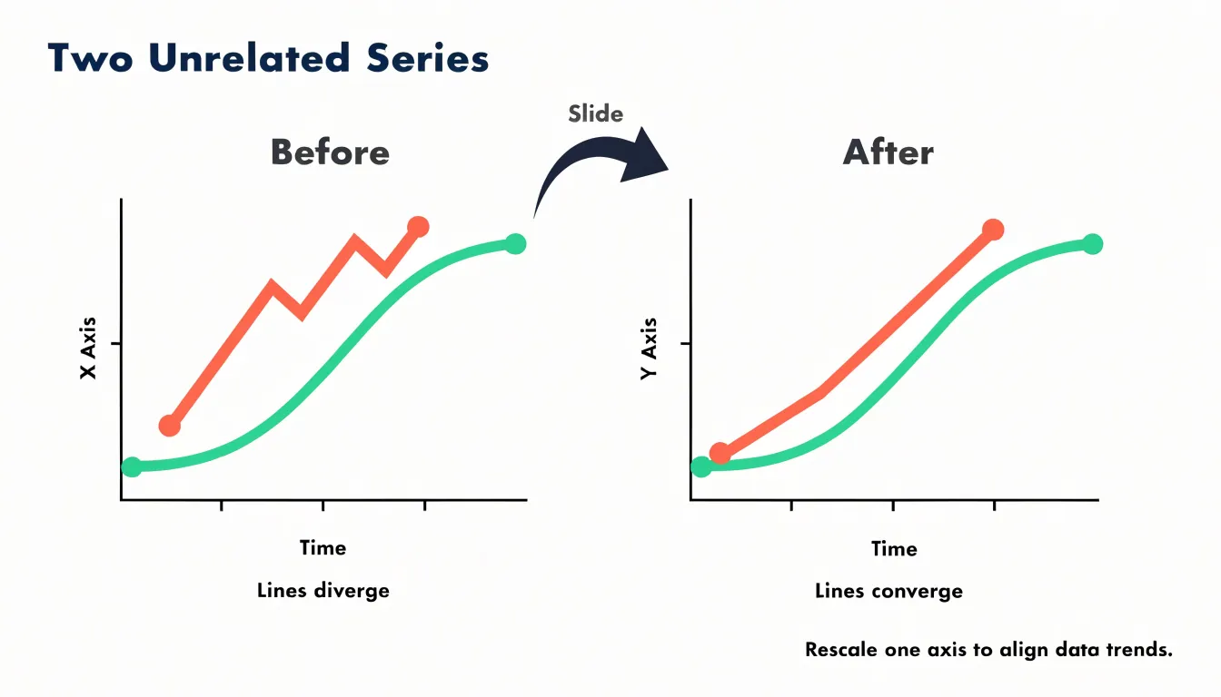
Unlinked dual axes present two separate data series on a single chart, each governed by its own independent y-axis scale. Because neither axis shares a common unit or baseline, the chart author has nearly unlimited freedom to position the two lines relative to one another. Sliding one scale up or down, or compressing and stretching its range, changes the visual relationship between the series entirely without altering the underlying data. An analyst hoping to show that two metrics move together can simply tune the axes until the lines overlap.
The manipulation works because the human eye reads spatial proximity and tandem movement as correlation and causal linkage. With unlinked axes, that synchrony is an artifact of axis design rather than a property of the data. A series measured in millions can be made to trace the exact path of a series measured in percentages purely by choosing ranges that force the shapes to coincide. Reverse the adjustment, and the same two datasets appear to diverge dramatically. Similarly, a rising line and a falling line positioned on opposing scales can manufacture an apparent inverse correlation.
Placing unrelated metrics on one chart implies a comparison the data cannot support, and few readers will reconstruct the original values to verify the relationship. A legitimate dual-axis chart, where the pairing is meaningful, labels both scales clearly, justifies the comparison, and typically anchors at least one axis at zero.
Improper Symbol Scaling
When a chart uses two-dimensional shapes—such as circles, squares, or icons—to represent quantities, the size of each shape must be scaled according to its total area rather than along a single linear dimension. Because area grows with the square of the linear dimension, doubling the height or diameter of an icon while keeping its proportions increases its total area fourfold. A value that rises by a factor of three produces a shape nine times heavier in area, and a factor of four produces a shape sixteen times heavier.
Because readers judge the visual bulk of a shape rather than measuring its diameter, linear scaling makes small differences in data look dramatic on the page. An already large value looks overwhelming, while a moderate value looks negligible.
To avoid this trap, designers must calculate the area required for each value and derive the corresponding radius or side length from that area, keeping every shape in the same proportions. Pairing a reference shape with a clear legend also helps readers calibrate their reading so the visual weight of each symbol corresponds faithfully to the data.
Oversized Pie Charts
While flat two-dimensional pie charts already strain the limits of human angle judgment, three-dimensional pie charts introduce severe distortion through perspective geometry and viewing angle tilt. Tilting a pie chart backward into the page places front slices closer to the viewer while back slices recede into the distance. Consequently, slices representing identical percentages appear dramatically different in size depending on where they land on the circle.
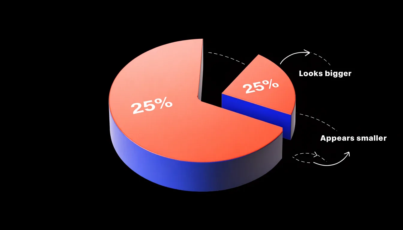
A front slice occupies more apparent vertical space, with a wider curved outer edge. A back slice is compressed by foreshortening, squeezing its arc into a shallower curve and shrinking its surface area on screen. Two slices each representing 25 percent of the total can look like one is a third of the pie and the other a mere sixth.
The extruded side walls of a 3D pie compound the problem. These edges add visible color that does not correspond to any data value, and the amount of this phantom area varies with position: front slices display tall, prominent walls, while back slices show almost none. Because viewers process perspective cues automatically and read the total colored region (walls included) as the slice’s magnitude, tilting or rotating the chart to move a slice toward the front shifts the apparent ranking of categories without changing the numbers.
Unequal Category Sizes
Unequal category sizes occur when a bar chart or histogram combines intervals of different widths, producing bars that appear comparable while summarizing very different spans of data. A histogram of ages might place years 0–5 in one bin, 5–18 in the next, and 18–65 in a third. Because each bar’s height reflects a total count rather than a rate, wider bins naturally accumulate more observations, meaning the tallest bar often reflects bin width rather than where data truly cluster. The same problem arises with time intervals: placing monthly figures beside quarterly and annual totals invites false comparisons, as a three-month quarterly bar will typically tower over a monthly bar simply by aggregating more activity.
This distortion works in two directions: wide bins manufacture apparent peaks by sweeping large swaths of a distribution into one category, while narrow bins make substantial groups look negligible. The true shape of the distribution—its skew, gaps, and clusters—is masked because every comparison of height carries a hidden denominator.
Correcting the problem requires aligning bin widths and intervals so every bar covers an equivalent range, or plotting rates and densities normalized to the width of each category. Where mixed intervals are unavoidable, clear labeling and separate panels help prevent false comparisons.
Misleading Color Choices
Color carries emotional weight before a reader processes a single number. Rendering a modest uptick—such as a two percent shift within normal variance or a seasonal fluctuation—in saturated alarm red taps into instinctive associations with danger and emergency. Because red draws the eye first, a line that would read as neutral in gray becomes a crisis in crimson. Furthermore, through the mere-exposure effect, repeated red treatment of a single category trains audiences to fear it.
Artificial contrast thresholds compound this effect. By coloring values above or below an arbitrary cut point in stark reds and greens, a chart manufactures the appearance of a dramatic binary divide where the data actually shows a gentle gradient. A cluster of points just past the threshold glows like a hazard sign, while nearly identical points on the other side look benign, even when the threshold reflects nothing meaningful about the data.
Even when statistics are accurate and axes are properly scaled, emotionally loaded palettes can impose a narrative of panic onto data that warrants calm reading. Careful chart design uses restrained, semantically consistent color and reserves high intensity for changes that genuinely deserve attention.
Ignoring Population Sizes
Choropleth maps that shade regions by raw counts rather than per capita rates largely reproduce the distribution of the population itself. Densely populated metropolitan areas inevitably appear as dark hotspots simply because more people live there, generating more hospital admissions, reported crimes, or new business registrations. Viewers read the dark shading as a concentrated problem, even when the underlying rate is unremarkable or lower than in sparsely populated rural districts that appear pale. The map measures density of people while appearing to measure density of risk.
The same failure applies to comparative rankings. A league table listing states, countries, or hospitals by total counts will almost always place the largest jurisdictions at the top, inviting the conclusion that they are the worst performers. Decision-makers relying on raw totals may channel resources toward large populations that are faring well proportionally, while overlooking small places with genuinely elevated rates.
Constructing a fair per capita measure requires a sensible denominator:
- Resident population for crime or disease
- Registered vehicles for traffic collisions
- Student enrolment for school incidents
Readers should treat any shaded map or ranking built on raw totals with suspicion until they confirm that population size has been accounted for.
Selective Data Smoothing
Selective data smoothing makes a chart tell a friendlier story by plotting a rolling average across a window of several periods instead of raw observations. A three-month or twelve-month moving average inevitably flattens sharp movements by diluting each extreme value with the calmer values on either side of it. When a wide smoothing window is chosen deliberately, a dramatic spike spread across twelve data points loses most of its visual height and disappears into a gently undulating line.
This conceals volatility that often carries the most important information in a dataset: a sudden drop in sales, a cluster of safety incidents, a surge in complaints, or a one-off operational failure. The casual viewer has no way of knowing that the reassuringly stable picture is an artifact of calculation rather than a property of the data.
Wide moving windows also shift and blur timing. Because a rolling average attributes past values to the current period, the visual peak of a smoothed line lags behind the actual event, obscuring when something went wrong. When the window size is undisclosed or changed between versions of a chart, authors can selectively present whichever degree of flattening produces their desired impression.
Misplaced Trend Lines
When a chart adds a straight arrow or a fitted linear regression line across a series of points, viewers instinctively read that line as a summary of the past and a forecast of the future. However, many real-world phenomena—such as sales figures, temperature readings, and stock prices—move in non-linear cycles, plateaus, and irregular swings. Fitting a straight line over wavy data manufactures a trend by averaging away the fluctuations that define the series.
For instance, in a metric that peaks and declines every few years, a straight line drawn across the full span may slope gently upward, suggesting steady growth even when the latest data point sits in the middle of a downswing. Conversely, linear averaging can produce a downward arrow through seasonal data that are actually stable or growing.
Projecting a linear regression line beyond non-linear data compounds the deception. Because the line’s slope reflects an arbitrary average of past ups and downs rather than the mechanism driving the series, the forecast fails sharply when the cycle turns. Trend indicators must respect the shape of the data: moving averages, seasonal decomposition, or plotting the raw series without an imposed line preserve cyclical signals without summarizing a pattern that does not exist.
Essential Checklist
Applying a five-step checklist takes under a minute and catches the errors that mislead readers most often:
- Inspect the axes. Read the horizontal and vertical labels to confirmwhether the units—such as percentages, thousands, or index points—match the claim being made.
- Locate the baseline. Confirm that bar charts begin at zero, and check whether non-zero starting points on other charts are justified by the data or chosen to exaggerate a gap.
- Check the scale. Look for uneven tick spacing, truncated ranges, or broken axis symbols that compress or stretch the data. Verify that logarithmic scales are clearly labeled.
- Trace the source metrics. Check the footnote or caption for the dataset name, time period, and sample size. Treat charts citing vague organizations or undated surveys with suspicion, and cross-check headline numbers against underlying figures where possible.
- Sanity-check the visual proportions. Compare the height of bars, area of shapes, or slope of lines against the printed numbers to ensure a doubled value does not look four times as large.
Frequently Asked Questions
What is a truncated y-axis?
A truncated y-axis starts the vertical scale at a value higher than zero, compressing the visible plotting area into a narrow band and exaggerating change. It can make a small fluctuation look like a dramatic surge or collapse.
How can I spot a misleading chart axis?
Check whether the vertical scale starts at zero, confirm that tick-mark intervals are consistent, and compare the visual change with the labeled start and end values. Also calculate the percentage change against the axis range to see whether the bounds are informing or persuading.
Why should bar charts start at zero?
Because the human eye compares the full lengths of bars from the baseline, so omitting zero distorts the visual ratio between categories. If two values are 100 and 110, starting the axis at 95 can make the second bar appear three times as tall instead of 10% taller.
What is an inverted scale in a chart?
An inverted scale flips the vertical axis so higher numerical values sit at the bottom and lower values sit at the top. It can make a declining trend look like growth because viewers associate upward motion with more.
Why do cumulative growth charts always seem to go up?
Cumulative charts plot a running total, so every new data point adds to everything before it and the line almost always rises even if current activity has slowed or reversed. They are appropriate for long-run totals, not for showing current momentum.
How can choosing a timeframe make a chart misleading?
Selecting start and end points carefully can hide a broader trend and create a false impression of stability, growth, or decline. A short window can obscure seasonal cycles or long-term context, so readers should check whether the date range represents the full history.
Tony Astor
Tony writes about data visualization and the tools people use to build charts and dashboards. More about Data Illustrator