Log Scale Explained: How to Read a Logarithmic Chart
 By Tony Astor ·

Log Scale Explained
A log scale spaces tick marks by a constant multiplier instead of a constant increment, so each equal step represents a fixed factor (10× on a base-10 axis). Equal vertical distances show equal percentage changes, turning exponential growth into a straight line and letting values spanning many orders of magnitude share one readable chart.
Table of Contents
Log Scale
On a log scale, the distance between any two adjacent tick marks corresponds to a constant multiplier rather than a constant increment. If the axis is built around base 10, each equal step upward represents a tenfold increase: the values run 1, 10, 100, 1000, and so on, yet the physical gap between each pair of labels stays the same. A base-2 axis works the same way with a factor of 2, stepping through 1, 2, 4, 8, 16. The reader’s job is to recognize this repeating multiplier and use it to decode position.
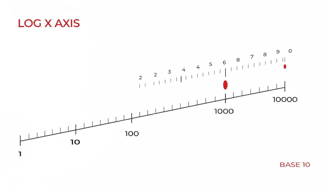
Reading a value begins with locating the nearest labeled tick and then counting the intermediate gridlines or minor ticks, each of which carries that same multiplicative factor. A point sitting one minor step above 100 on a base-10 axis reads as 1000; a point one step below 100 reads as 10. Because the factor is constant, the same visual distance always translates to the same proportional change, whether the reader is near the bottom of the axis or near the top.
This structure makes proportional growth legible at a glance. On a linear axis, a jump from 10 to 20 and a jump from 1000 to 1010 occupy very different amounts of space, even though the first is a doubling and the second is a rounding error. On a log axis, a doubling always spans the same distance, so a curve that climbs at a steady slope reflects steady percentage growth. Readers tracking exponential trends, compound interest, or population changes can compare the steepness of lines directly, since equal slopes mean equal growth rates. The axis rewards attention to ratios and factors, and it lets values spanning many orders of magnitude share a single readable frame.
Linear vs. Log Scale
When you place two graphs side by side, one with a linear axis and the other with a logarithmic axis, the same dataset can look strikingly different. On a linear scale, equal distances represent equal absolute changes. A curve that grows exponentially will bend upward ever more steeply, compressing early values near the bottom and stretching later values toward the top. Switch to a log scale, where equal distances represent equal multiplicative factors, and that same exponential curve transforms into a straight line. This happens because taking the logarithm of an exponential function yields a linear relationship. The visual flattening is a powerful cue: if a curve straightens out on a log axis, the underlying process likely follows a power law or exponential growth.
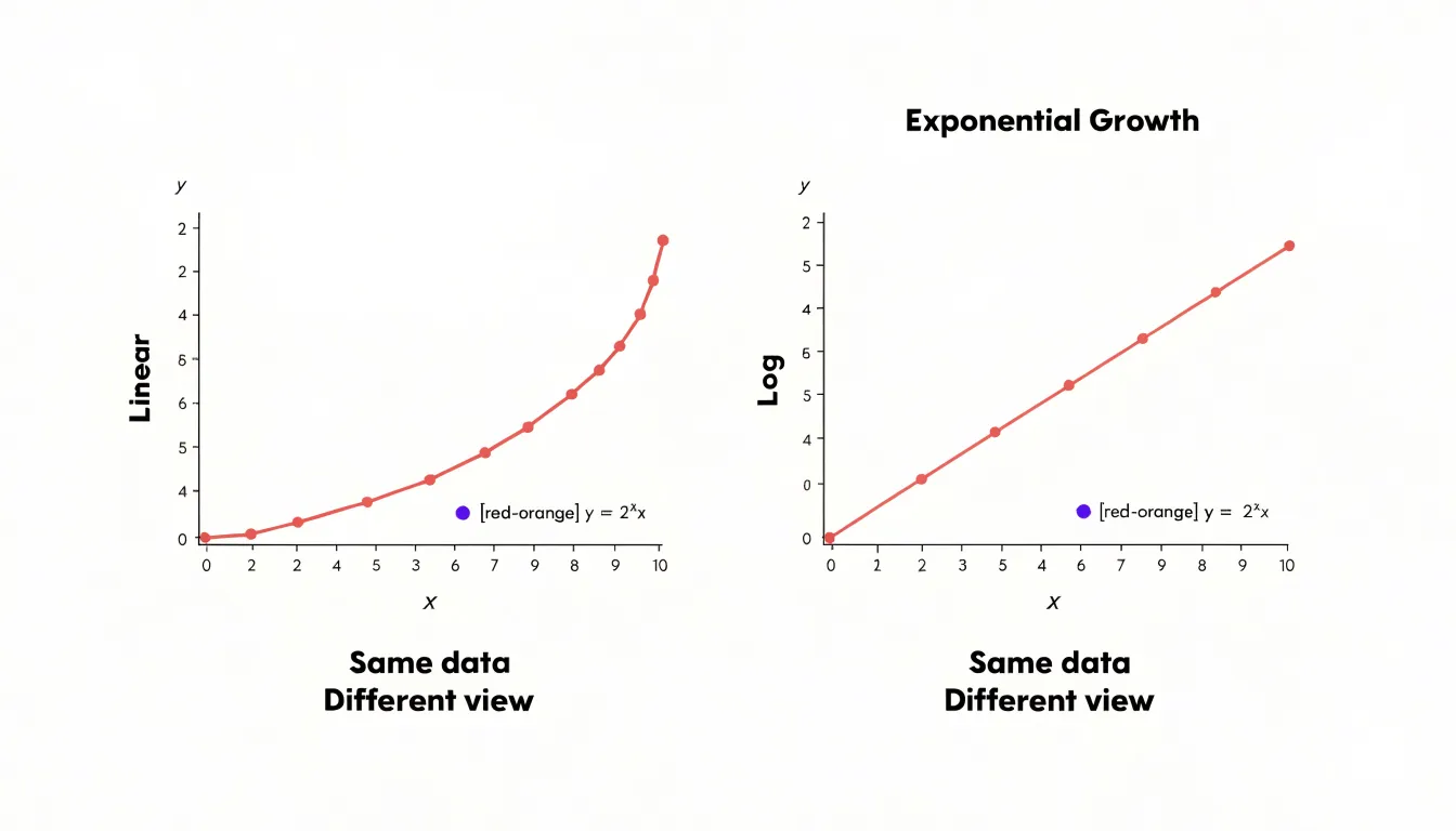
To spot these differences, start by examining the axis labels. A linear axis shows evenly spaced tick marks with constant increments, such as 0, 10, 20, 30. A log axis displays ticks that grow by a constant factor, such as 1, 10, 100, 1000, with wider gaps at the low end and tighter gaps at the high end. Next, look at the shape of the data. On a linear plot, a straight line indicates a constant rate of change. On a log plot, a straight line indicates a constant percentage rate of change. Curves that appear to flatten or saturate on a linear scale may reveal continued growth when plotted on a log scale.
Before analyzing trends, check for these visual cues: the spacing of grid lines, the presence of minor tick marks between major ones, and whether the vertical axis includes a break or starts at zero. A log scale never includes zero, so any plot with a log axis will begin at a positive value. Also, note that the same data can appear to have different slopes depending on the scale. Always confirm the axis type before drawing conclusions about growth rates or comparing series. Side-by-side comparisons make these differences obvious and help you avoid misinterpreting the story your data tells.
Orders of Magnitude
Every log chart rests on the idea of an order of magnitude, which is simply a way of describing numbers in terms of powers of ten. Instead of counting in fixed increments of one, ten, or a hundred, an order-of-magnitude view asks how many times ten must be multiplied together to reach a given value. The number 100 is two orders of magnitude above 1 because 10 × 10 = 100. The number 1,000 sits three orders above 1, and 10,000 four orders above. Each step of ten represents the same multiplicative jump, whether the values involved are tiny fractions or enormous figures.
This regularity is the mathematical foundation of base-10 log charts. Because each power of ten corresponds to a single equal step on the axis, a chart can move from 1 to 10 to 100 to 1,000 without changing the spacing between tick marks. The physical distance on the page maps directly onto the exponent: an exponent of 1 sits one unit to the right of an exponent of 0, an exponent of 2 sits one unit beyond that, and so on. The visual result is a steady rhythm of evenly spaced increments that stand for multiplicative change.
The practical payoff appears when data spans a wide numerical range. Values running from single digits up to millions would flatten most of a linear chart into an unreadable smear near the bottom, with the largest points towering far above everything else. By condensing each power-of-ten jump into a single manageable visual step, a log scale brings those extremes into a workable frame. Growth that multiplies tenfold appears as the same rise as any other tenfold multiplication, so patterns of proportional change become visible across the entire range of the data.
Log Scale Grid Lines
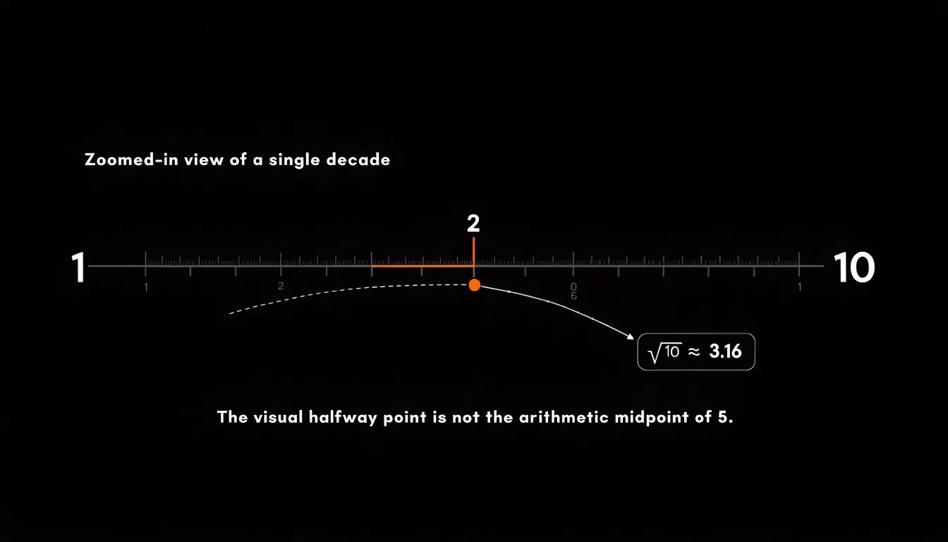
Log Scale Grid Lines — navigating non-uniform spacing. On a log scale, the distance between major grid lines marks equal multiplicative steps, usually powers of ten. The space between 1 and 10 is identical to the space between 10 and 100, yet the values inside each interval behave very differently. Tick marks that subdivide the interval sit at 2, 3, 4 and so on times the lower bound. Because the scale compresses higher numbers, these ticks crowd together as they approach the next order of magnitude. The gap from 2 to 3 is visibly wider than the gap from 8 to 9, even though both represent a change of one unit. Near the top of the interval, the lines bunch up tightly, while near the bottom they spread out generously. Reading a log chart accurately means internalizing this rhythm. A useful habit is to locate the halfway point of each interval. On a log scale, the midpoint between 1 and 10 sits at roughly 3.16, the square root of ten, rather than at 5. From there you can halve the remaining space again to find about 10, and continue subdividing. When estimating a value that falls between labeled ticks, judge its position relative to the surrounding lines rather than assuming even spacing. A point that appears to sit a quarter of the way from 10 to 100 is actually near 17.7, since the visual distance corresponds to a multiplicative factor. Another practical tip is to count the minor lines when they are present; many charts show ticks at every integer multiple, which gives you anchor points to interpolate against. With a little practice, the uneven spacing becomes a reliable visual language, letting you read magnitudes and ratios directly off the page instead of misjudging values by treating the grid as linear.
Exponential Data
Exponential processes grow by a constant multiplicative factor over each interval, so their values can climb from a handful of cases to many thousands within a short span of time. A viral outbreak that doubles every three days, or a bacterial colony that doubles every twenty minutes, produces a sequence of measurements where the early values are tiny relative to the later ones. Plotted directly on a standard linear axis, the same curve that begins with a few dozen infections and reaches millions will show its first weeks compressed into a nearly flat line hugging the baseline, with almost no visible detail. Every early data point sits so close to zero that differences between twenty and forty cases, which matter enormously for detecting the start of an outbreak, become indistinguishable to the eye.
Applying a logarithmic scale to the vertical axis resolves this by spacing values according to their orders of magnitude rather than their absolute differences. Each equal step on the axis represents the same multiplicative factor, so the gap between one and ten occupies the same vertical distance as the gap between one hundred and one thousand. When exponential data are plotted this way, a constant growth rate appears as a straight line, and deviations from that line become immediately visible. Analysts can read the doubling time directly from the slope, compare the trajectories of different regions or strains side by side, and spot the moment when growth begins to slow as an upward curve bending toward the horizontal.
The practical technique is straightforward. Choose a logarithm base suited to the data, often base ten for case counts spanning several powers of ten or base two when doubling behavior is the focus, and label the axis in the original units so readers can still read raw values. Keep the axis starting from a meaningful minimum such as one case rather than zero, since the logarithm of zero is undefined. With these settings, the earliest measurements remain legible, and the full arc of the outbreak or colony growth can be examined on a single chart without losing the critical early signal.
Constant Percentage Change
A straight line on a log graph indicates a constant percentage change, which is the hallmark of steady relative growth. To see why, consider that the vertical axis on a log graph is scaled so that equal distances represent equal multiplicative factors—for example, each unit might correspond to a tenfold increase. When a quantity grows by a fixed percentage each period, its logarithm increases by a constant amount. This is because the logarithm of a product equals the sum of the logarithms, so repeated multiplication by a constant factor translates into repeated addition of a constant. On a log graph, that constant addition produces a straight line with a slope proportional to the growth rate.
This property makes log graphs powerful for distinguishing compound growth from other patterns. Exponential growth, where the absolute increase accelerates over time, appears as a straight line on a log graph. In contrast, linear growth—where the quantity increases by a fixed absolute amount each period—curves downward on a log graph because the percentage growth rate declines as the quantity gets larger. Similarly, growth that is faster than exponential would curve upward.
By spotting a straight sloped line, readers can quickly conclude that the underlying process is growing at a steady relative rate, such as a fixed interest rate, a constant inflation rate, or a population increasing by a consistent percentage each year. The slope of the line directly reflects the size of that percentage change: a steeper slope means a higher growth rate. This visual shortcut allows for rapid comparison of growth rates across different series and helps identify periods of stable exponential growth within noisy data.
Comparing Large and Small Numbers
When metrics span many orders of magnitude, a linear axis struggles to serve every value at once. Conceive of a dataset where the smallest observation is measured in fractions of a unit while the largest climbs into the millions. On a conventional plot, those micro readings collapse into a flat line hugging zero, their variations invisible, while a handful of macro values stretch the vertical space and force everything else into the bottom margin. A log scale resolves this by compressing each order of magnitude into an equal interval, so the distance between 1 and 10 matches the distance between 1,000 and 10,000. The consequence is that the full spectrum of values occupies a workable span on a single page. Lower-tier values retain room to spread and reveal their own patterns, fluctuations, and relative differences, no longer flattened into a single indistinguishable cluster. At the same time, extreme outliers remain within the plot area because each successive tenfold increase consumes the same amount of vertical room as the last. Nothing needs to be clipped or excluded to keep the chart readable, and no value gets drowned out by the sheer size of its neighbours. This simultaneous display of micro and macro readings is especially useful in fields where variation at both ends carries meaning: transaction amounts in financial data, population counts across regions, signal strengths, or concentrations in scientific measurement. Readers can compare a value near the bottom of the range with one near the top using the same visual language, since equal vertical steps always represent equal multiplicative changes. The page holds the entire range intact, letting small and large figures coexist without one erasing the other.
Semi-Log vs. Log-Log
When you encounter a graph with a logarithmic scale, one of the first things worth establishing is which axis carries the transformation. A semi-log graph applies a logarithmic scale to one axis, typically the vertical one, while the other axis remains linear. A log-log graph applies a logarithmic scale to both axes. This structural difference determines what kinds of relationships each graph is built to reveal.
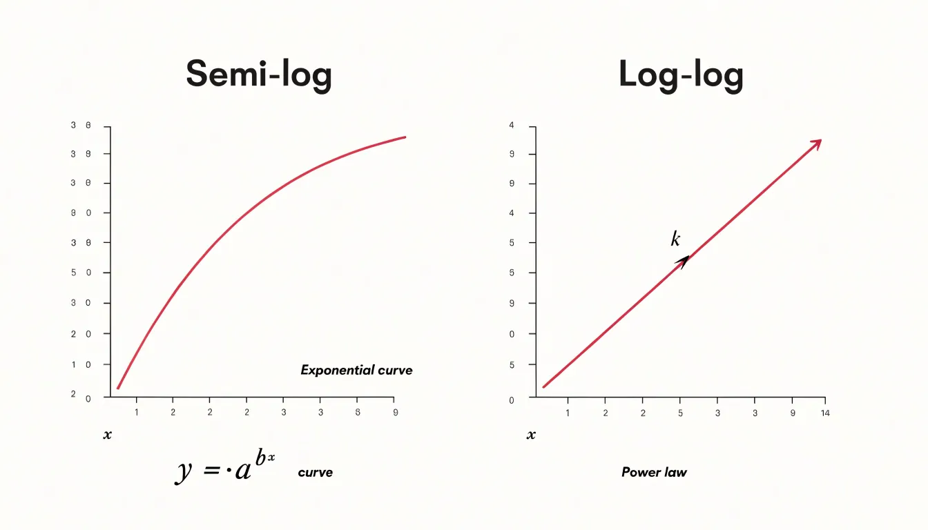
In a semi-log plot with a logarithmic y-axis and a linear x-axis, a straight line corresponds to exponential growth or decay. This happens because taking the logarithm of an exponential function, such as y equals a times b to the power of x, produces a linear equation in log y and x. Each equal step along the linear axis multiplies the value on the log axis by a constant factor. This makes semi-log graphs the natural choice for phenomena like compound interest, population growth, radioactive decay, or bacterial doubling, where the quantity changes by a fixed percentage per unit of time rather than by a fixed amount.
In a log-log plot, both axes are scaled logarithmically, and a straight line indicates a power-law relationship of the form y equals a times x to the power of k. The slope of that line corresponds directly to the exponent k, so the graph makes the strength and direction of the relationship easy to read. Power laws appear throughout the natural and social sciences, from the distribution of earthquake magnitudes and city sizes to scaling laws in biology and physics.
The practical rule follows from these structures. When your data involves multiplicative change against an additive variable, a semi-log graph will straighten the curve. When both variables span several orders of magnitude and you suspect a power-law connection, the log-log graph exposes that structure. Matching the graph type to the underlying relationship keeps the visual pattern interpretable and the analysis grounded.
Real-World Log Scales
Logarithmic scales appear throughout applied science because they solve a practical problem: many natural phenomena vary across ranges so vast that a linear scale becomes unusable. The Richter scale, developed to describe earthquake magnitude, illustrates this clearly. Seismic energy released by earthquakes spans many orders of magnitude, from faint tremors to catastrophic ruptures. By taking the logarithm of measured ground motion amplitudes, seismologists compress this enormous range into manageable numbers. A magnitude 6 earthquake releases roughly thirty times more energy than a magnitude 5, and each whole-number step corresponds to a consistent multiplicative increase. This standardization lets scientists, emergency planners, and the public compare events quickly without wrestling with raw amplitude figures in the millions.
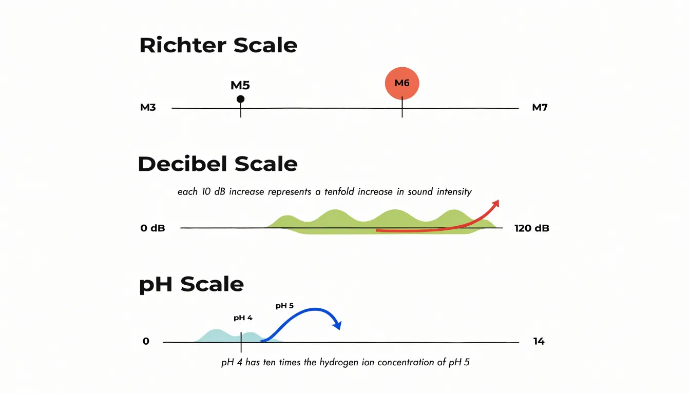
Acoustic decibels follow the same logic. The human ear perceives sound intensity across a range from the faintest audible whisper to the roar of a jet engine, a span of roughly a trillion units of power. Measuring sound pressure directly would produce unwieldy numbers, so acoustics uses a logarithmic ratio. Each increase of ten decibels represents a tenfold rise in sound intensity. This convention aligns with how hearing actually works, since perceived loudness grows roughly with the logarithm of physical intensity. Engineers designing concert halls, audiologists fitting hearing aids, and safety regulators setting workplace noise limits all rely on this standardized scale to communicate levels that would otherwise be impractical to express.
The pH scale in chemistry applies the same principle to hydrogen ion concentration. Acidity can range from extremely concentrated strong acids to very dilute solutions, and the relevant concentrations often differ by factors of millions or more. Expressing concentration as the negative logarithm of hydrogen ion activity compresses this range into the familiar zero-to-fourteen scale. A pH of 4 indicates ten times the hydrogen ion concentration of pH 5. Chemists, biologists, and water quality technicians use pH daily to describe soil conditions, blood chemistry, and drinking water safety with compact, comparable values. Each of these scales shows how logarithms turn sprawling measurement ranges into standards usable in laboratories, clinics, and everyday decision-making.
Financial Charts
Logarithmic price charts serve stock market investors by representing equal percentage changes as equal vertical distances, which makes them indispensable for studying long-term market trends. On a standard linear chart, a move from $10 to $20 occupies the same vertical space as a move from $1,000 to $1,010, even though the first is a doubling of capital and the second is a gain of just one percent. When an investor examines several decades of price history on such a chart, the early years compress into a flat line near the bottom while recent years dominate the picture, and this distorted perception can lead to poor decisions about asset allocation and risk.
A logarithmic scale corrects this problem by spacing gridlines according to multiplicative rather than additive increments. A doubling of price always spans the same vertical distance, whether it occurs in 1985 at $5 per share or in 2020 at $500 per share. This property lets investors compare percentage returns across widely separated eras on a consistent basis. A fifty percent decline during a bear market in the 1970s appears with the same visual steepness as a fifty percent decline in the 2000s, which helps investors recognize recurring patterns of boom and bust without being misled by the nominal price level of the moment.
Long-term investors also use log charts to assess whether a trend has genuinely accelerated or merely continued at a steady compounding rate. A constant growth rate plots as a straight line on a log scale, so any deviation from that line signals a meaningful change in momentum. This makes log charts a practical tool for evaluating whether decades-long uptrends remain intact and for setting expectations about future returns grounded in compounding rather than in absolute dollar figures.
Common Reading Mistakes
Log scales compress large ranges into compact visual space, and that compression changes how a chart reads at a glance. A frequent mistake is interpreting the steepness of a line on a log axis as if it showed absolute change. On a linear chart, a steep segment usually means values are rising quickly in raw terms. On a log chart, slope reflects proportional or percentage change, so a line that looks dramatic may represent a modest absolute increase when the underlying counts are small, while a visually gentle line at the top of the chart may hide a very large absolute swing. Readers who carry linear habits into log charts often overestimate the severity of upticks near the bottom of the scale and underestimate changes among large values. This produces misread spikes, where an outbreak or revenue bump appears alarming or trivial depending on where it sits on the axis rather than on what the numbers actually say. A practical checklist helps prevent this. First, confirm whether the axis is logarithmic or linear, since many tools label ticks in powers of ten without saying so explicitly. Second, read the tick values rather than trusting the spacing, because equal visual gaps represent multiplicative steps. Third, trace any apparent spike back to the underlying numbers to see whether the change is absolute or proportional. Fourth, check whether the axis starts at a value greater than zero, which can exaggerate visual movement. Fifth, compare rates of change rather than slopes when comparing series. Finally, when spikes matter, cross-check against a linear version of the same chart to see how the two views differ. Building these checks into routine chart reading keeps visual drama from being mistaken for real magnitude.
Software Tools
Most spreadsheet and graphing packages treat a logarithmic axis as a display setting layered on top of ordinary data, so the workflow stays the same regardless of which tool you open. In Microsoft Excel, begin by selecting your chart and opening the Format Axis pane, usually by right-clicking the axis and choosing Format Axis. Within the Axis Options section, locate the checkbox labeled Logarithmic scale and tick it. Excel offers a Base field beside the checkbox, defaulting to 10, which you can change to 2 or any other value if your data calls for it. Confirm the axis labels still make sense, since Excel may reset minimum and maximum bounds when the scale changes; adjust those bounds manually in the same pane if the chart looks squeezed.
Google Sheets follows a nearly identical path. Double-click the chart to open the Chart Editor, switch to the Customize tab, and expand the Vertical axis or Horizontal axis section depending on which axis you want to transform. A Log scale checkbox appears there, again paired with a base selector. Clicking it redraws the chart immediately, and you can fine-tune the axis minimum and maximum in the adjacent fields.
In Python’s Matplotlib, the adjustment happens in code rather than a menu. Call ax.set_xscale(‘log’) or ax.set_yscale(‘log’) on the relevant axis object, optionally passing a base argument such as base=2. For quick plots, plt.xscale(‘log’) works the same way. After setting the scale, review tick placement; Matplotlib handles major and minor ticks automatically but may need ax.set_xlim() or ax.set_ylim() to frame the data well. Across all three tools, the underlying principle holds: enable the log toggle, verify the base, and inspect the resulting tick labels before sharing the chart.
Chart Literacy
Log scales reward careful reading, and that reading is a skill anyone can build. When you finish exploring a log-scaled chart, you should come away with a practical toolkit for interrogating any visualization that crosses your path. Start by locating the axes. Check whether the gridlines represent equal increments or constant ratios; the spacing of labels reveals which world you are in. Look at where the baseline sits, and ask what happens to the story if the scale were linear. Scan for the small annotations, axis titles, and unit labels that often carry the key to interpretation. Ask what the vertical distance between two points represents: on a log axis, a fixed gap corresponds to a fixed percentage change, so equal-looking steps can encode very different absolute shifts. A modest rise near the top of the chart may reflect the same proportional growth as a large-looking climb near the bottom. Practice reading a handful of values directly off the grid and comparing them with your quick visual impression. This habit trains you to separate genuine trends from artifacts of scale choice. Media charts frequently compress or stretch axes to dramatize a point, and a reader who notices unequal increments, truncated baselines, or unlabeled logarithmic axes can judge whether the emphasis is honest. The same discipline helps with dense dashboards and scientific figures crowded with multiple series and shaded bands. Slow down, trace one series at a time, and translate each visual gap into a ratio. Over time these checks become automatic, and you gain the confidence to critique charts in news articles, spot misleading scale decisions, and extract reliable insights from even the most complex visual data.
Frequently Asked Questions
What is a log scale used for?
A log scale spaces tick marks by a constant multiplier rather than a constant increment, so equal visual steps represent equal multiplicative factors. It makes proportional growth and values spanning many orders of magnitude readable at a glance.
How do you read values on a log scale?
Find the nearest labeled tick and count the intermediate gridlines or minor ticks, since each carries the same multiplicative factor. For example, on a base-10 axis, one minor step above 100 reads as 1000.
What is the difference between a linear scale and a log scale?
On a linear scale, equal distances represent equal absolute changes; on a log scale, equal distances represent equal multiplicative factors. This is why an exponential curve can bend upward on a linear axis but appear as a straight line on a log axis.
Why does exponential data appear as a straight line on a log scale?
When exponential data are plotted on a log scale, a constant growth rate appears as a straight line. Analysts can read the doubling time from the slope and spot deviations from that line more easily.
What does a straight line on a log graph mean?
A straight line on a log graph indicates a constant percentage change, such as steady relative growth. In contrast, linear growth curves downward on a log graph because its percentage growth rate declines as the quantity gets larger.
Can a log scale start at zero?
No; a log scale never includes zero because the logarithm of zero is undefined, so a log axis begins at a positive value. When plotting exponential data, the article says to keep the axis starting from a meaningful minimum such as one case rather than zero.
Tony Astor
Tony writes about data visualization and the tools people use to build charts and dashboards. More about Data Illustrator