Linear vs Log Scale: When to Use Each
 By Tony Astor ·
Linear vs Log Scale
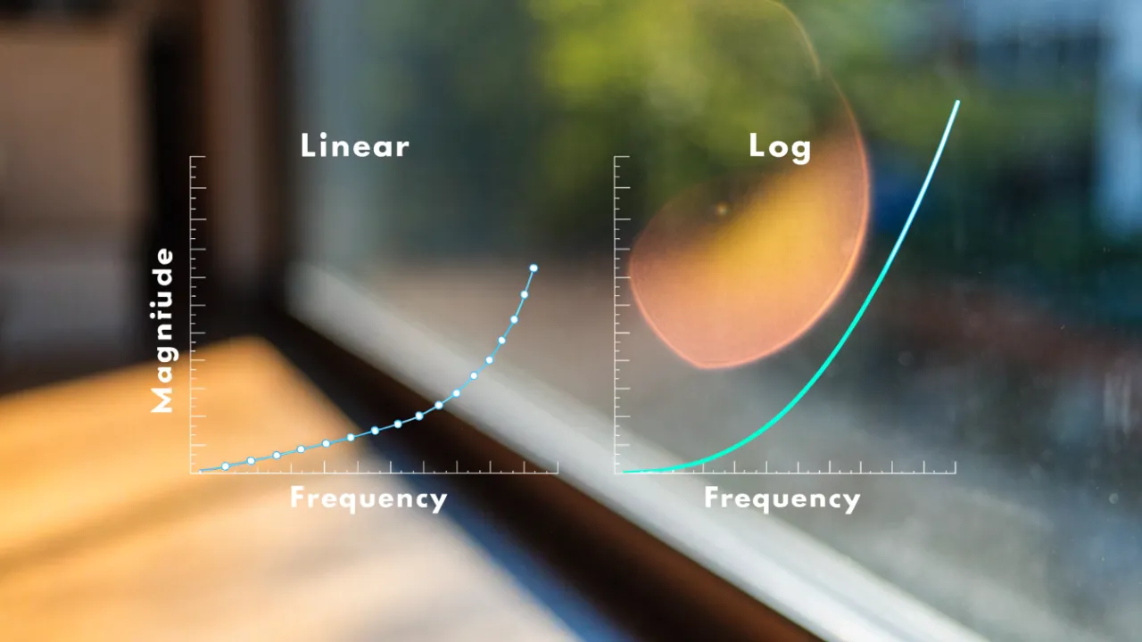
A linear scale spaces values by equal addition, so equal distances represent equal absolute changes, while a log scale spaces values by multiplication, so equal distances represent equal percentage changes. Use linear for steady data and log for exponential growth, wide ranges, or ratios spanning orders of magnitude.
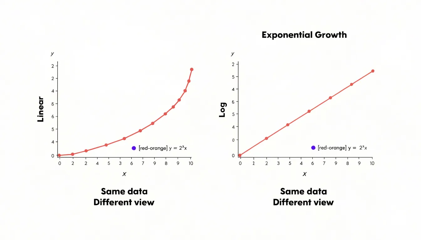
Table of Contents
- Linear Scale
- Log Scale
- Handling Huge Spikes
- The Magic of Multiples
- Reading Logarithmic Spacing
- Tracking Investment Returns
- Pandemic and Disease Spreads
- Sound Waves and Earthquakes
- Managing Massive Ranges
- Common Graphing Pitfalls
- Smart Axis Labeling
- Setting Up Digital Charts
- Communicating with Clarity
- Practical Chart Selection
Linear Scale
A linear scale represents values by mapping equal physical distances on the axis to equal additive increments. If one unit of measurement corresponds to one centimeter of space on a chart, then every additional centimeter represents exactly one more unit, regardless of where you are along the axis. Moving from 2 to 3 covers the same distance as moving from 12 to 13, because the scale advances by constant addition rather than by multiplication. This one-to-one correspondence between distance and quantity gives the linear scale its characteristic even spacing, with tick marks appearing at regular intervals from the origin outward.
This structure makes the linear scale the natural choice for data that change in steady, uniform amounts. Consider height: someone growing from 150 to 160 centimeters adds ten centimeters, and that increase occupies the same visual span as a jump from 170 to 180 centimeters, so the chart reflects the actual physical change with direct proportionality. Daily step counts behave the same way. A person logging 5,000 steps and then 10,000 steps has doubled their activity, and the linear axis shows that gap as one fixed block of distance, while a day with 2,000 additional steps appears as a visibly smaller increment. Readers can compare differences simply by measuring the length of the segments between points, since every segment of equal length represents an equal absolute change.
Because linear scales count step by step, they preserve the intuitive sense of magnitude that people bring to everyday quantities. A bar twice as tall stands for a value twice as large, and an increment of a fixed size always looks the same. For steady, uniform data such as height, weight, distance, or daily step totals, this direct correspondence keeps absolute differences visible and comparisons straightforward, letting the chart speak in the same additive terms as the underlying measurements.
Log Scale
On a log scale, each grid mark represents a multiplication factor rather than a fixed addition. The distance between 1 and 10 is the same as the distance between 10 and 100, and the same again between 100 to 1,000. Every step along the axis corresponds to multiplying by ten, so the ticks might read 1, 10, 100, 1,000 rather than 0, 100, 200, 300. That construction means equal visual distances always correspond to equal percentage changes, no matter where you are on the chart.
This is the key to understanding what a log scale is really measuring. When a value climbs from 100 to 200, that is a 100% increase. When it climbs from 1,000 to 1,100, that is a 10% increase, even though the absolute jump is five times larger. A linear scale treats both jumps according to their raw size, so the second change dominates the picture. A log scale treats them according to their proportional size, so the 100% move stands out while the 10% move looks modest. Each grid mark now stands for a multiplication factor, and the eye reads distance as rate of change in percentage terms.
This makes log scales well suited to quantities that grow by compounding, where each period’s increase builds on the last. Population growth, investment returns, viral spread, and inflation all behave this way. Percentage-based spacing keeps the early, smaller values visible while still accommodating the later, much larger ones. A value that doubles repeatedly traces a straight line on a log chart, which makes constant growth rates easy to spot. The result is a view that highlights proportional motion, showing how fast something is changing relative to where it started.
Handling Huge Spikes
When a dataset contains a sudden geometric increase, a linear axis has to stretch itself to accommodate the largest value, and that stretch happens all at once across the entire chart. The vertical scale is divided into equal steps from zero to the peak, so a spike of, say, ten thousand units forces the axis to run from 0 to 10,000. Every smaller value in the series is then drawn against that same grid. A reading of fifty units, which may represent an important early trend or a meaningful baseline, becomes a sliver so close to the horizontal axis that it is visually indistinguishable from zero. A reading of two hundred units climbs only a tiny fraction of the chart height. The result is a graph where the spike dominates the picture and the rest of the data collapses into a flat, unreadable line hugging the bottom edge.
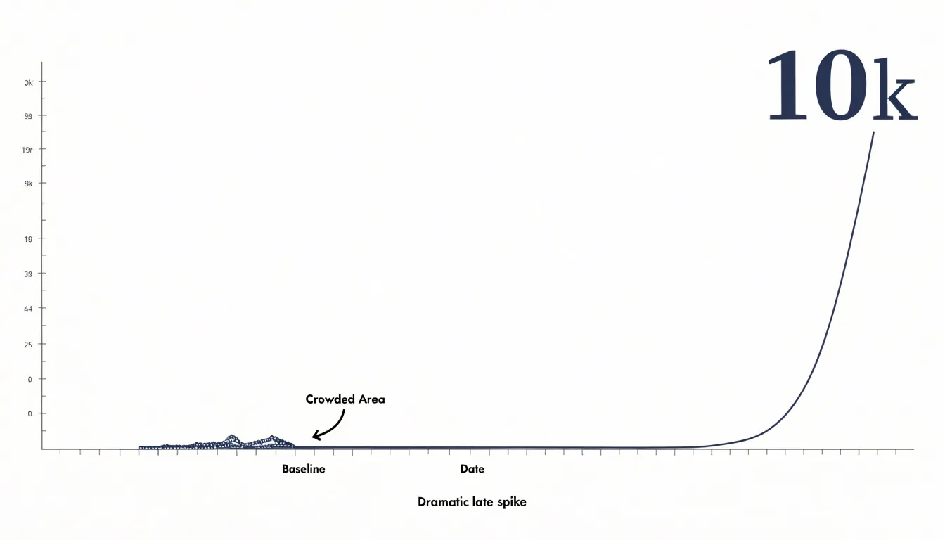
This compression is a direct consequence of equal spacing. Linear graphs allocate the same physical distance to every fixed increment, whether that increment is 10 or 10,000. Once the axis is scaled to the maximum, small differences that matter enormously in context occupy almost no vertical room. Analysts looking at such a chart can see that a dramatic jump occurred, yet they cannot see the shape of the data before it. Subtle movements, gradual buildups, and ordinary fluctuations all disappear into the same crowded band near zero.
The practical difficulty is that the most interesting information often lives in exactly that crowded band. Early growth, seasonal variation, and the moment a trend begins to accelerate are all small relative to a later spike. On a traditional linear axis those details are flattened by the scale itself, and the reader is left with a chart that communicates magnitude but hides structure. Recognizing this limitation is the first step toward choosing a presentation that preserves both the spike and the smaller movements around it.
The Magic of Multiples
A logarithmic scale transforms the way we perceive numerical differences when those differences span several orders of magnitude. On a linear scale, the distance between 1 and 10 is the same as the distance between 10 and 19, and a value of 1,000 would require a chart a thousand times longer than one showing 1. This becomes impractical when plotting data like earthquake magnitudes, population sizes, or financial values that range from thousands to billions. By spacing orders of magnitude uniformly, a log scale allows a single chart to display values as small as 0.001 and as large as 1,000,000 without any one value overwhelming the rest.
The magic lies in how this compression preserves relative patterns while shrinking giant gaps. On a linear scale, a value of 1,000,000 would dwarf a value of 1,000, making the smaller value invisible. On a log scale, both appear with the same visual separation as 1 and 10. This makes it possible to compare growth rates, identify exponential trends, and spot outliers across vastly different scales. The human eye can then discern patterns that would otherwise be lost in a sea of empty space or clustered at the bottom of the chart. Moreover, log scales handle ratios naturally: a doubling of value always occupies the same vertical distance, regardless of the starting point. This is why log scales are indispensable in fields from microbiology to astrophysics, where data routinely span many orders of magnitude.
Reading Logarithmic Spacing
On a logarithmic axis, the distance between tick marks shrinks as the numbers grow larger. The gap from 1 to 2 occupies a wide stretch, the gap from 2 to 3 is noticeably narrower, and by the time you reach 8, 9, and 10 the lines crowd together into a tight band. This clustering is a direct consequence of how logarithms compress values: each tick represents an equal multiplicative step, so doubling from 1 to 2 covers the same vertical distance as doubling from 50 to 100. Understanding this rhythm is the key to reading the scale accurately.
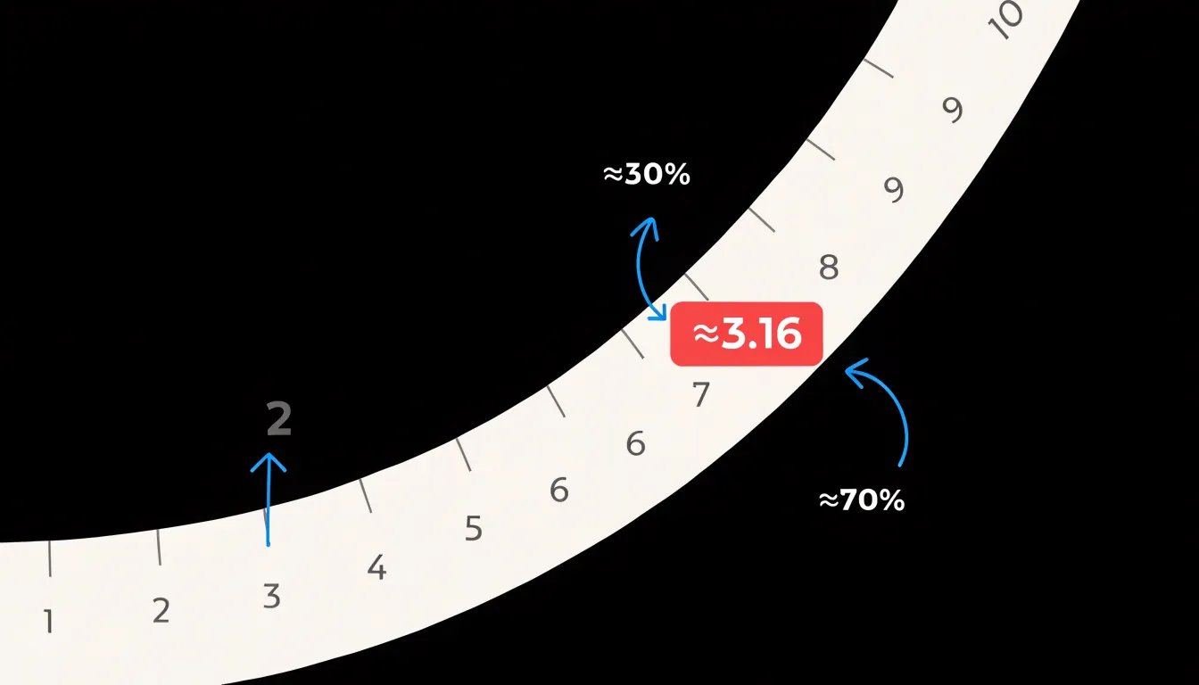
A useful habit is to anchor yourself on the major powers of ten first. Locate 1, 10, 100, and 1000 and note that the space between each consecutive pair is identical. Everything in between follows the same repeating pattern of clustering, so once you have learned the shape of one decade, you can read any other decade on the chart with the same intuition. The midpoint of a decade, for instance, sits at roughly 3.16 rather than 5, because the halfway mark in log space corresponds to the square root of ten. Knowing a few of these landmarks, such as 2 sitting about 30 percent of the way along the decade and 5 sitting about 70 percent of the way, lets you place intermediate values quickly.
When estimating a value that falls between two labeled ticks, interpolate within the local spacing rather than assuming an even division. If a point lies halfway between the 3 and 4 marks, it represents about 3.5, since the spacing there is still reasonably wide. Near the crowded upper end of a decade, however, small visual distances correspond to larger numeric jumps, so treat estimates between 8 and 10 with more caution. With practice, the non-uniform lines become a familiar map rather than an obstacle, and you can read magnitudes off the axis with confidence.
Tracking Investment Returns
Logarithmic scales are the gold standard for visualizing portfolio growth because they represent proportional changes consistently across all price levels. On a log chart, a 10% gain occupies the same vertical distance whether the underlying value is one hundred dollars or one million dollars. For investors, this means a 10% return on a small account early in a career appears identical in magnitude to a 10% return on a large portfolio decades later. Such consistency allows meaningful comparison of performance across time and across different asset sizes.
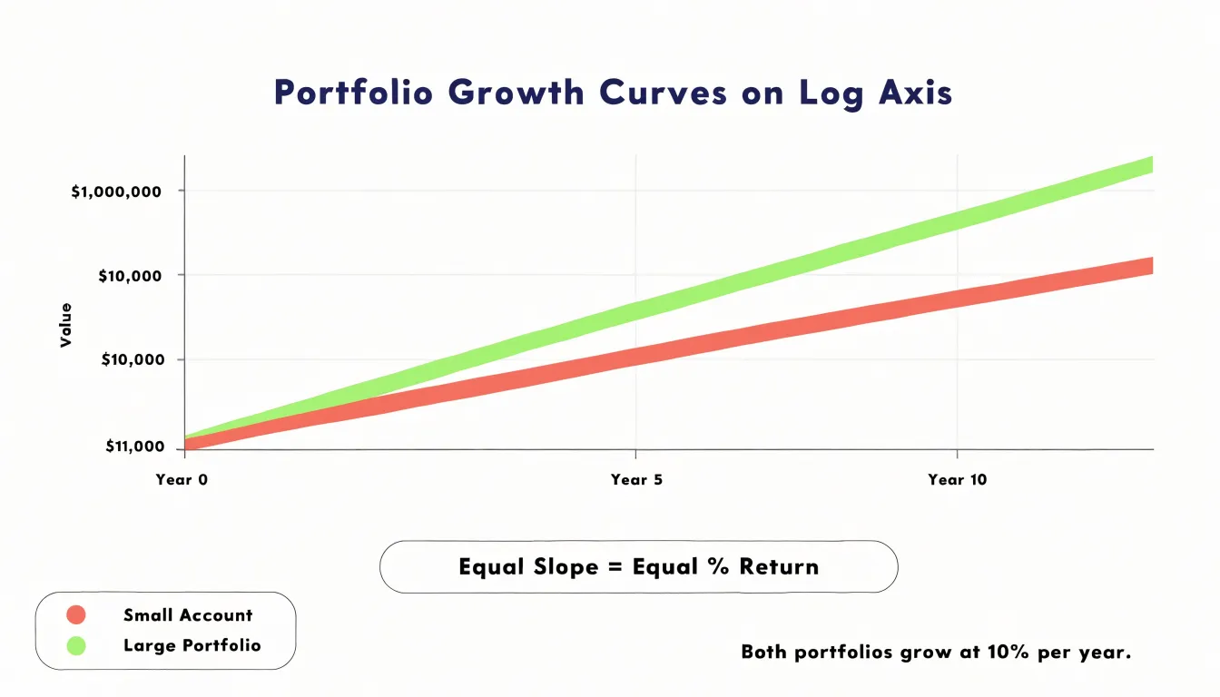
When tracking compounding interest, linear charts can distort perception. A linear chart shows absolute dollar changes, so a $1,000 gain on a $10,000 portfolio seems ten times larger than a $100 gain on a $1,000 portfolio, even though both represent a 10% return. This visual bias can mislead investors into overemphasizing recent, larger absolute gains while underestimating the impact of early percentage returns. A log chart eliminates this distortion by focusing on the rate of growth rather than the dollar amount. The slope of the line on a log chart directly indicates the growth rate: a steeper slope means a higher percentage return per unit time, regardless of the portfolio’s absolute value.
Because log scales make exponential growth appear as a straight line—the true signature of compounding—investors can easily assess whether their portfolio is growing at a steady rate or if the growth rate is accelerating or decelerating. By normalizing the visual representation for percentage changes, a log scale lets financial analysts compare the performance of different assets or strategies on a level playing field over the long term.
Pandemic and Disease Spreads
During a disease outbreak, public health analysts face a daunting task: making sense of case counts that can grow at a staggering pace. In the early stages of an epidemic, the number of infections can double every few days, producing figures that climb so rapidly on a standard linear chart that the line shoots almost straight up. This kind of visualization obscures the finer details of transmission dynamics, because the eye is drawn to the overwhelming vertical climb rather than the underlying rate of change.
On a log chart, exponential growth appears as a straight, upward-sloping line, and the steepness of that line corresponds directly to the transmission rate. Analysts can therefore compare the growth trajectories of different regions or time periods at a glance, and a slope that begins to bend downward signals that the rate of new infections is slowing. This early signal of curve flattening is often difficult to detect on a linear plot, where a slowdown can be masked by the sheer volume of accumulated cases.
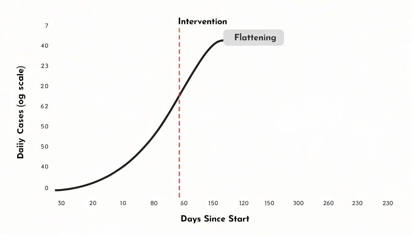
Log scales also help evaluators judge the effectiveness of interventions such as mask mandates, school closures, or vaccination campaigns. When a policy takes effect, a sustained reduction in the slope of the log-scale line provides evidence that transmission is decelerating, even while absolute case numbers remain high. By translating explosive growth into a readable, comparable form, log scales give public health analysts a clearer view of how a pandemic unfolds and how well countermeasures are working.
Sound Waves and Earthquakes
Sound waves and seismic waves share a characteristic that makes logarithmic scales indispensable: their intensity ranges span many orders of magnitude. The decibel scale, used to measure sound, is a logarithmic ratio that compares a sound’s intensity to a reference level. The human ear perceives loudness in roughly logarithmic fashion, meaning that a tenfold increase in sound intensity is heard as a doubling of loudness. This is why the decibel scale is so practical: it compresses an enormous range of physical intensities into a manageable set of numbers. A whisper might be around 30 decibels, normal conversation around 60 decibels, and a rock concert around 120 decibels. Each 10-decibel increase represents a tenfold increase in intensity, yet our ears hear these steps as roughly equal increments in loudness. The decibel thus aligns physical measurement with sensory perception, making it a natural tool for engineers and audiologists alike.
Similarly, the Richter scale, developed by Charles Richter in the 1930s, quantifies the energy released by earthquakes. It is a base-10 logarithmic scale, so each whole number increase corresponds to a tenfold increase in measured amplitude and roughly 31.6 times more energy release. An earthquake of magnitude 5 is ten times more powerful in amplitude than one of magnitude 4, and about 32 times more energetic. This logarithmic compression allows seismologists to describe everything from faint tremors to catastrophic quakes on a single, readable scale. Without it, the numbers would be unwieldy and difficult to compare.
Both scales illustrate how logarithmic ratios emerge naturally when measuring phenomena that span wide dynamic ranges. They also show that our perceptual systems and our measurement tools often converge on logarithmic representations because they are efficient and intuitive. In daily life, we encounter these scales in weather reports, music volume settings, and earthquake news, often without realizing the mathematical principle at work. Understanding the logarithmic nature of these scales helps us interpret the numbers correctly and appreciate why a small numerical change can mean a huge difference in physical intensity.
Managing Massive Ranges
Managing massive ranges in a dataset requires deliberate choices about how space is allocated across the chart. When values span several orders of magnitude, a linear axis compresses the smallest observations into a sliver near the origin, so a change from 0.1 to 0.5 becomes visually indistinguishable from no change at all. Converting equal ratios into equal distances on a logarithmic axis gives minor baseline fluctuations their own visible territory while still leaving room for extreme values at the top of the scale. A small percentage shift near the bottom of the range occupies as much visual space as the same percentage shift near the top, allowing readers to track subtle movements in low-magnitude series alongside dramatic swings in high-magnitude ones.
Handling outliers is a related concern. A few extreme observations can stretch the axis so far that the bulk of the data collapses into a narrow band. Options include:
- Log transforms that naturally dampen outlier influence.
- Symlog scales that behave linearly near zero and logarithmically beyond a threshold.
- Axis breaks that skip a region of the scale while flagging the discontinuity.
Each approach trades some interpretability for retaining detail in the dense part of the distribution.
Annotation and context matter as much as scale selection. Labeling decades or key thresholds on the axis helps readers calibrate their reading of distance, and providing a reference series or trend line keeps the baseline interpretable when the scale itself is non-linear. Interactive zooming paired with an overview panel lets viewers inspect fine-grained fluctuations without sacrificing the global picture. Consistency across related charts also prevents misreading, since switching scale between panels of the same figure invites false comparisons. The goal throughout is a layout where neither end of the range disappears.
Common Graphing Pitfalls
Scaling choices shape what a reader actually sees long before any numbers are examined. A chart that truncates the vertical axis so it begins above zero can turn a modest two percent change into a dramatic visual cliff, because the eye compares the height of the bars or the slope of the line rather than the underlying quantities. This is the most familiar pitfall, yet it remains common in quarterly reports and marketing materials precisely because it produces an impressive picture at a glance. The same distortion appears when the aspect ratio of a chart is stretched or compressed; widening a line chart flattens volatility, while narrowing it manufactures sharp swings out of ordinary noise. Logarithmic axes introduce their own hazards: because a log scale compresses large values and expands small ones, readers who expect equal spacing to mean equal increments will misread the magnitude of early changes. A steep-looking climb on a log axis may represent steady percentage growth rather than accelerating growth, and labels that omit the word log leave the audience to assume linear spacing by default.
Spotting these problems requires a few quick checks:
- Look for axis labels that start at a number other than zero on a bar chart, since bars encode magnitude through length and therefore demand a true baseline.
- Examine whether the tick intervals are equal and clearly marked, because missing or irregular ticks often accompany cherry-picked ranges.
- Check the caption and axis title for a stated scale type, and be suspicious of charts where small absolute differences appear as towering columns.
- Compare the visual change against the stated percentages; if the picture suggests a doubling while the numbers show a five percent move, the range has been chosen to exaggerate.
- Note whether the horizontal axis covers the full period relevant to the claim, since cutting off earlier data can make a recovery or decline look sharper than it is.
Recognizing these signs lets readers separate genuine trends from artifacts of presentation.
Smart Axis Labeling
Clear gridlines provide essential reference points, helping viewers estimate values without guesswork. On a logarithmic scale, gridlines should align with major powers of ten (1, 10, 100, 1000) and include minor lines for intermediate values, all labeled consistently. This structure allows non-technical audiences to grasp the multiplicative nature of the scale.
Scale indicators, such as a clear label like ‘Logarithmic Scale (base 10)’ near the axis, remove ambiguity. Annotations further guide interpretation: a note explaining that an upward curve on a log plot indicates exponential growth at a constant rate prevents the common misconception that the curve is merely steep. For exponential data, highlighting key milestones (e.g., ‘value doubles every 10 units’) reinforces understanding. Consistent labeling across all axes and series ensures that comparisons are valid and transparent. When presenting to a general audience, consider adding a brief explanatory subtitle or a small inset describing how to read the scale. These practices keep the data honest by avoiding visual distortion and approachable by bridging the gap between statistical rigor and everyday intuition.
Setting Up Digital Charts
Setting up a digital chart with logarithmic axes begins with locating the axis formatting options in your chosen tool:
- Microsoft Excel: Start by creating a standard chart from your data range, then right-click the vertical axis and choose Format Axis. A side panel opens where the Axis Options section contains a checkbox labeled Logarithmic scale; checking it applies base-10 logarithms by default, and the adjacent box lets you specify a different base such as 2 or the natural base. Repeat the process for the horizontal axis if your x-values span several orders of magnitude.
- Google Sheets: Open the Chart Editor, switch to the Customize tab, expand the Vertical axis section, and tick the Log scale box. The Horizontal axis section offers the same control. Both Excel and Google Sheets rescale tick marks automatically, so verify that your data contains only positive values, since logarithms of zero or negative numbers cannot be plotted and will be dropped.
- Matplotlib (Python): Use the
plt.yscaleandplt.xscalefunctions, where passing the string'log'converts the corresponding axis, or call theset_xscaleorset_yscalemethods on an Axes object to achieve the same result. - Seaborn: Because it inherits Matplotlib’s behavior, calling
set(xscale='log')on a plot or passinglog_scalearguments to relational and categorical plotting functions works cleanly. - Plotly: Assign
type='log'inside the layout dictionary for each axis.
Across all these environments, a final review of labels and tick formatting helps readers interpret the compressed upper range and expanded lower range that a logarithmic axis produces.
Communicating with Clarity
When presenting data on a log scale, start by explicitly stating that the scale is logarithmic and explain what that means in plain terms. For example, you might say, ‘This chart uses a log scale, which means each major grid line represents a tenfold increase.’ Avoid jargon like ‘orders of magnitude’ unless you define it immediately. Use captions that highlight the scale and its implications, such as ‘Note: Log scale—equal distances represent multiplicative changes.’ In presentations, consider adding a simple visual aid, like a side-by-side comparison of linear and log scales for the same data, to illustrate the difference.
When explaining trends, focus on relative changes rather than absolute differences. For instance, ‘Sales grew from 100 to 1,000, a tenfold increase’ is clearer than ‘Sales increased by 900 units.’ Use analogies familiar to your audience, such as comparing the scale to the Richter scale for earthquakes, which many people know is logarithmic. Encourage questions and provide a brief explanation of why a log scale was chosen—perhaps to show both small and large values clearly. Build trust by being transparent about the transformation and its purpose, and avoid overwhelming your audience with technical details. For written reports, include a short explanatory paragraph or a footnote. In interactive dashboards, tooltips can explain the scale when users hover.
Practical Chart Selection
Choosing between a linear and a logarithmic view becomes straightforward when you turn the decision into a short sequence of questions:
- Check the range: Ask whether the values span only one or two orders of magnitude or climb across three or more. When the range is narrow and evenly behaved, a linear axis keeps distances intuitive and lets readers compare heights directly. When the values stretch across many orders of magnitude, a log axis compresses the upper end and gives the smaller values room to show their shape.
- Check the variance pattern: Data with steady absolute increments suit a linear scale, while data that grows by consistent percentages, compounds over time, or swings wildly across periods reads more clearly on a log scale.
- Check the audience: A general audience arriving without a quantitative background will move through a linear chart with little explanation, while a log chart may invite misreadings of equal visual gaps. A technical or analytical audience already familiar with log axes can absorb the compressed view and will often expect it for growth or ratio data.
- Check the core message: If the point is that one category dwarfs another, a linear scale dramatizes that gap and makes the disparity obvious. If the point is that growth rates are comparable or that small values still matter, a log scale surfaces those patterns that a linear view would flatten.
When the answers point in different directions, show both views side by side and label them clearly, letting the comparison itself carry the argument.
Frequently Asked Questions
What is the difference between a linear scale and a log scale?
A linear scale maps equal physical distances to equal additive increments, so moving from 2 to 3 covers the same distance as moving from 12 to 13. A log scale uses each grid mark as a multiplication factor, so equal visual distances correspond to equal percentage changes.
When should I use a log scale instead of a linear scale?
Use a log scale when values span several orders of magnitude, grow by compounding, or change by consistent percentages over time. A linear scale is natural for steady, uniform data such as height, weight, distance, or daily step totals.
Why do small values look flat on a linear chart with a huge spike?
A linear axis must stretch from zero to the peak, and equal spacing is allocated to every fixed increment, so smaller values are compressed near the horizontal axis. This can make important early trends, baselines, and ordinary fluctuations visually indistinguishable from zero.
How do you read a logarithmic scale?
Anchor yourself on the major powers of ten first, since the space between each consecutive pair is identical, and note that tick marks cluster together as the numbers grow larger. The midpoint of a decade sits at roughly 3.16, and values between labeled ticks should be interpolated within the local spacing rather than assuming an even division.
Why do investors use log scales to track portfolio returns?
On a log chart, a 10% gain occupies the same vertical distance whether the underlying value is one hundred dollars or one million dollars. The slope of the line on a log chart directly indicates the growth rate, so a steeper slope means a higher percentage return per unit time.
How do I set up a log scale in Excel or Google Sheets?
In Excel, right-click the vertical axis and choose Format Axis, then check the Logarithmic scale box under Axis Options. In Google Sheets, open the Chart Editor, go to Customize, expand the Vertical axis section, and tick the Log scale box; both tools rescale tick marks automatically, so verify that your data contains only positive values, since logarithms of zero or negative numbers cannot be plotted and will be dropped.
Tony Astor
Tony writes about data visualization and the tools people use to build charts and dashboards. More about Data Illustrator