Line Chart vs Scatter Plot: Key Differences
 By Tony Astor ·

Line Chart vs Scatter Plot
Use a line chart to show how a value changes over an ordered sequence such as time, where connecting points reveals trend, rate of change, and momentum. Use a scatter plot to show how two variables relate across independent observations, preserving individual points to expose correlation, clusters, density, and outliers.
Table of Contents
Line Chart
A line chart is built around the idea that data points belong to a sequence, and that the sequence itself carries meaning. The x-axis is typically reserved for chronological values—dates, months, quarters, or timestamps—so that each marker sits at a defined moment in time. Once the points are placed in order from earliest to latest, the chart draws straight segments between them. These connecting lines state visually that the observations are linked, allowing a reader to follow the rise and fall of a metric across a period and see whether values are climbing, dipping, flattening out, or oscillating.
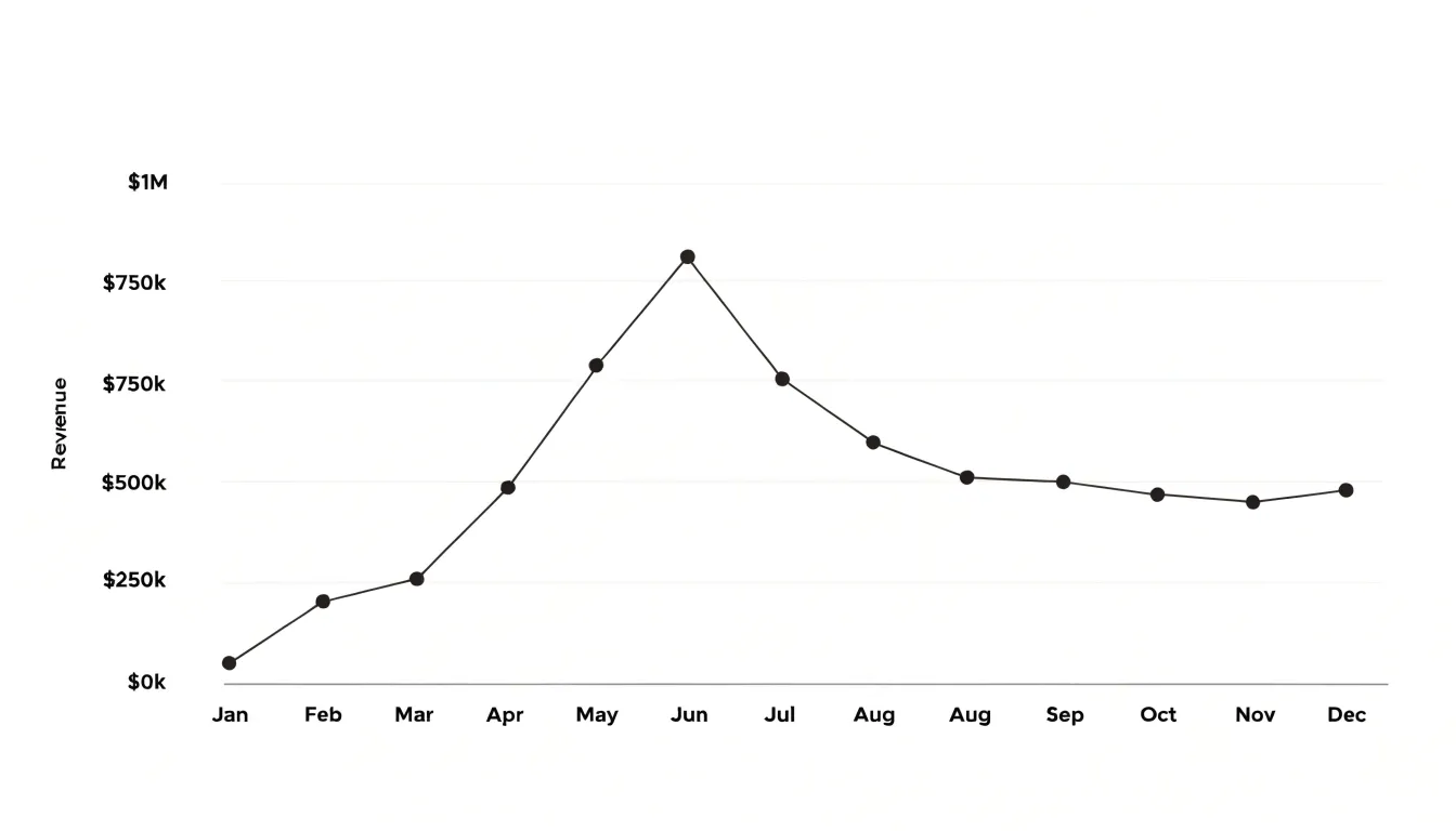
The slope of each segment encodes the rate of change: steep lines signal rapid movement, gentle lines suggest slower drift, and flat lines indicate stability. Because the line is continuous, the eye is pulled along the path, conveying temporal momentum—the sense that a trend is accelerating, losing steam, or holding steady. Connected points also make it easier to spot turning points, seasonal cycles, and sustained shifts that isolated markers would leave hidden.
The chronological order on the x-axis gives the chart its logic; without that sequence, the connecting segments would imply relationships that the underlying measurements may not support. When the goal is to show how a value evolves over time, the line chart offers a compact format that emphasizes flow and direction rather than isolated observations.
Scatter Plot
A scatter plot places each observation on a Cartesian plane according to its values on two numerical variables, with one variable assigned to the horizontal axis and the other to the vertical axis. Every dot represents a single data pair, and its position reflects the exact combination of measurements recorded for that observation. This arrangement lets a viewer inspect the full set of data pairs at once and observe how the values of one variable accompany the values of the other.
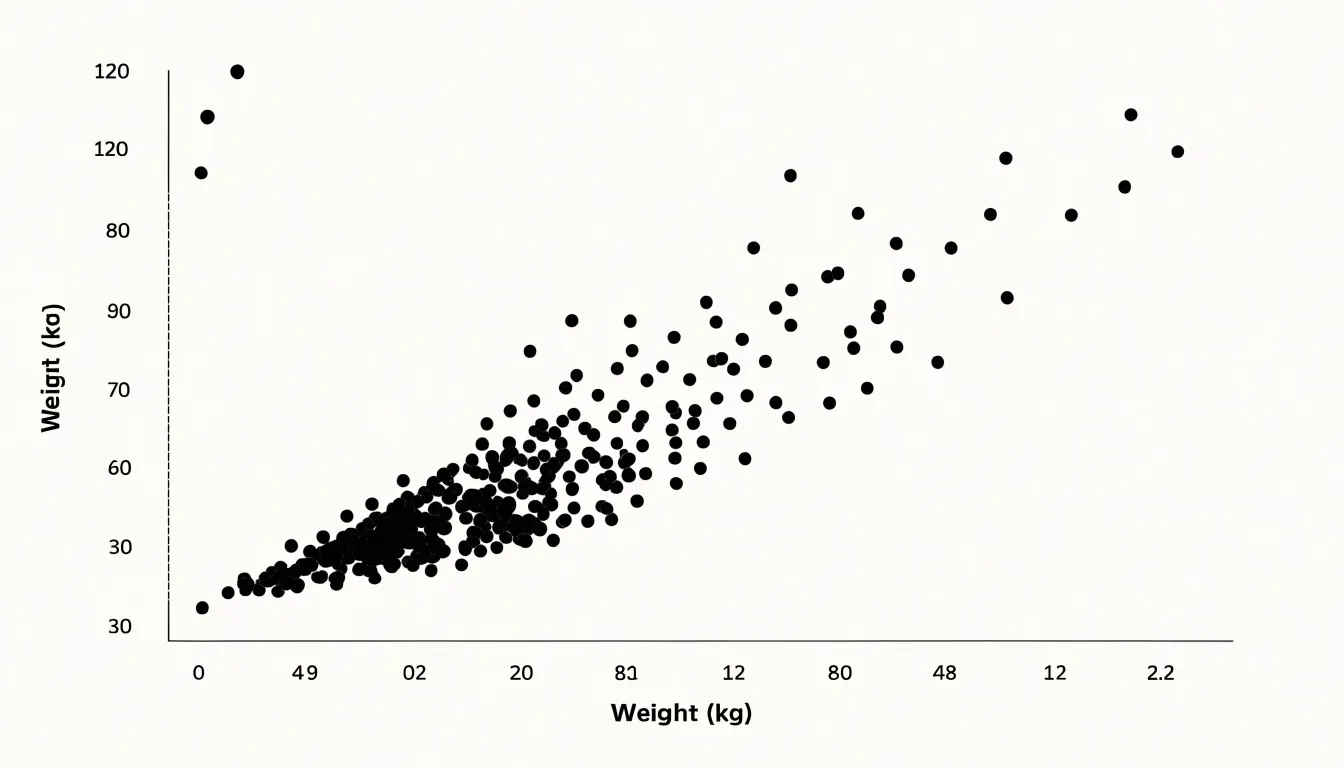
Patterns that remain hidden in tables or summary statistics often become visible in this layout, including clusters of similar observations, gaps where no data fall, and the overall direction in which the cloud of points stretches. Analysts read these features as evidence of association, correlation, or the absence of any systematic relationship. Outlying points also stand apart clearly, drawing attention to observations that may warrant closer investigation.
A scatter plot does not require observations to follow any sequence. The horizontal axis may hold a measurement such as temperature, age, or price, none of which implies a natural ordering of cases. Because the dots are placed solely by their coordinate values, the plot treats the data as a collection of independent pairs and makes no assumption about time or progression. This makes the scatter plot a foundational tool for exploratory analysis of paired measurements.
Line vs Scatter
The choice between connecting dots and leaving them apart stems from the mathematical nature of the data. A line chart assumes continuity: the variable on the horizontal axis progresses in an ordered sequence, and the line segment between two points represents the intermediate values that exist between them. This interpolation is meaningful when the underlying phenomenon is continuous—temperature over hours, stock prices over days, or distance over time. The line implies a rate of change and guides the eye along a path that mirrors causal or temporal flow.
A scatter plot treats each point as an independent observation. The horizontal axis often represents a variable that is not inherently ordered, such as height, income, or age, and there is no expectation that a straight line between two points corresponds to any real entity. Leaving points apart preserves the integrity of each datum and allows the overall shape, clustering, and correlation to emerge from the cloud of points itself.
A line chart emphasizes progression and how one value leads to the next. A scatter plot emphasizes distribution and how two variables co-vary across independent cases. Connecting dots in a scatter plot would impose a false sequence, turning a snapshot of a population into a misleading trajectory.
Line Chart
When tracking a single metric across fixed time intervals—such as monthly sales figures, daily website traffic, or quarterly revenue—consistent baselines allow viewers to quickly grasp the direction and magnitude of change. Line charts expose both short-term volatility and cyclical patterns, such as weekly sales spikes or annual seasonal dips.
To maximize clarity, follow these best practices:
- Space time intervals evenly: Uneven gaps distort the perception of trends.
- Label axes clearly: Include units, time increments, and a descriptive title stating the metric and timeframe.
- Use distinct line styles: Use solid lines for continuous historical data and dashed lines for projections, avoiding excessive decoration.
- Highlight recurring fluctuations: Add a trendline or shade specific periods (such as holiday seasons) to draw attention to seasonal patterns.
- Choose an appropriate y-axis baseline: Starting the y-axis at zero is generally recommended for ratio data to avoid exaggerating changes, though for metrics like temperature, a non-zero baseline may be appropriate.
Scatter Plot
Instead of reading individual values in isolation, a scatter plot reader evaluates the shape, direction, and density of the entire distribution to see how two factors move in relation to one another.
- Positive correlation appears as a pattern running from the lower-left region toward the upper-right. Points with small horizontal values tend to sit low on the vertical axis, while points with large horizontal values sit high. As one factor increases, the other tends to increase.
- Negative correlation produces the mirror image: the pattern descends from upper-left to lower-right, so larger values on one axis pair with smaller values on the other. When one factor rises, the other tends to fall.
- Zero correlation shows up as a shapeless cloud with no clear upward or downward drift, indicating that changes in one variable carry little or no information about changes in the other.
The density of the points matters as much as their direction. A tight, well-defined band signals a strong, consistent relationship across many observations, while a loose, widely spread formation suggests a weaker connection. Because a few outlying points can stretch or distort the visible pattern, it helps to scan the full field—reading direction, tightness, and outliers together—before drawing conclusions.
Line Chart
A line chart’s core strength in forecasting lies in how its historical slope provides a basis for projecting where future data points might fall. Extending the visible trajectory forward gives analysts a working estimate of future movement grounded in the observed behavior of the series.
Directional momentum reinforces this projection. A line that has climbed at a consistent angle over several periods suggests an established pattern likely to continue in the near term, while a gradually steepening slope signals that the rate of growth itself is increasing. These visual cues map directly onto forecasting techniques such as trend extrapolation, where the historical slope is used to estimate values beyond the last recorded point.
This approach works best with continuous time series where observations arrive at regular intervals and the underlying pattern evolves gradually. It also makes deviations easy to spot: a sudden break from the established slope stands out immediately and prompts a reassessment of the forecast.
Scatter Plot
The spatial structure of a scatter plot is the foundation for both outlier detection and cluster recognition. An outlier is an observation positioned far away from the main body of points, corresponding to a large deviation in the underlying values. Analysts typically begin by scanning visually for isolated points above, below, or to the side of the central grouping. Formalizing that judgment involves measuring each point’s distance from the center of the data:
- Z-scores on each axis, flagging points lying more than a set number of standard deviations from the mean.
- Mahalanobis distance, which accounts for the correlation between variables.
- Interquartile range (IQR) approaches, which offer a distribution-free alternative.
Clusters appear when points form distinct concentrations separated by sparser regions. Recognizing them begins with noting where point density rises and falls, and confirming that the separation is real rather than an artifact of sparse sampling. Analysts can quantify grouping through methods such as k-means or density-based clustering, then project the resulting group assignments back onto the plot through color or marker shape.
Interactive plotting aids this process: zooming and panning reveal structure that a static overview can hide, and brushing lets analysts select regions to inspect the corresponding records. Outlier detection and cluster recognition reinforce each other in practice, because a point that looks anomalous against the whole dataset may belong cleanly to a small sub-group, and a cluster boundary often clarifies which observations genuinely stand apart.
Line Chart
Line charts apply across diverse fields where tracking a value over consistent intervals matters:
- Meteorology: Weather stations record hourly temperature readings, forming curves that reveal warming afternoons, cooling evenings, and seasonal arcs.
- Finance: Traders and analysts track stock closing prices across days, weeks, or years to identify momentum, volatility, support levels, breakouts, and downturns.
- Operations and Healthcare: Organizations monitor website traffic across a quarter, energy consumption through the day, patient vital signs in a hospital, or production output across a fiscal year.
Scatter Plot
Scatter plots excel in research contexts that examine the relationship between two continuous variables measured on the same observational unit, preserving individual-level granularity rather than aggregating data into categories:
- Anthropometry: Plotting height on the horizontal axis against weight on the vertical axis for each individual reveals the direction, strength, and form of the physical association.
- Biomedical research: Investigators plot body mass index (BMI) against blood pressure across a cohort to assess whether higher BMI co-occurs with elevated pressure, while spotting outliers that warrant follow-up.
- Demographics: Plotting income against life expectancy across regions exposes gradients, clusters, and nonlinear patterns that summary statistics alone might obscure.
- Experimental and observational studies: Dose-response experiments, epidemiological surveys, and ecological monitoring use scatter plots to inspect variability, detect influential cases, judge whether a linear model is appropriate, and display fitted trendlines or confidence bands.
Axis Setup
Axis setup determines whether a chart’s visual proportions remain faithful to the underlying numbers.
- Baseline choice: A bar chart that starts its value axis at zero shows magnitudes in true proportion, while a truncated axis exaggerates small differences. Line charts tracking continuous change sometimes justify a non-zero baseline to make meaningful variation visible, but that decision should be deliberate and disclosed because readers anchor on where an axis begins.
- Axis intervals: Evenly spaced tick marks labeled at a sensible frequency let viewers translate vertical distance into quantity with confidence. Irregular or unexplained jumps compress some regions of the plot and stretch others, making equal changes appear unequal.
- Aspect ratio: The frame’s proportions determine the visual slope of every trendline. A wide, short frame turns a dataset into a gentle drift, while a tall, narrow frame turns identical numbers into a steep climb. For time series data, analysts often default to a ratio near 4:3 or 16:9, keeping it fixed across comparable charts.
- Scatter plot scaling: Each axis should scale to the data’s actual range with enough padding to prevent points from crowding the frame edges, and both axes should follow the same conventions throughout a set.
Common Mistakes
Drawing a line between data points that have no meaningful order or progression is a persistent charting error. Because a line implies that the horizontal variable moves continuously and that intermediate values are real, applying it to unordered data misleads the viewer.
This problem appears most often when the horizontal axis is categorical. Suppose a chart compares sales across product categories such as shoes, hats, and jackets. Connecting these points with a line implies that sales travel through the space between shoes and hats. Because the categories are discrete and unordered, the slope reflects nothing more than an arbitrary arrangement of labels; reorder the categories and the line changes shape entirely.
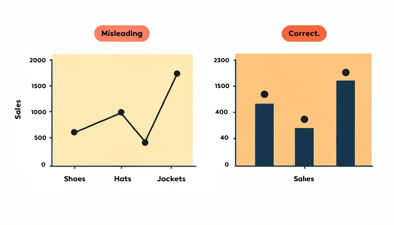
A related pitfall involves joining non-sequential numerical data. Connecting independent scatter observations in the order they were recorded creates zigzags that look like volatility or cycles, when they only trace the sequence of data entry.
Lines also invite visual interpolation. When a viewer sees a segment between two points, the mind assumes the value halfway along is approximately halfway between the endpoints. For categorical data or scattered observations, no halfway value exists. Reserve lines for data with a genuine continuous ordering, and let unordered comparisons stand as bars or dots.
Multiple Data Sets
When a chart carries multiple data sets, combining visual encodings prevents overlapping series from blending together:
- Color coding: Assign a distinct hue from a perceptually even palette to each series so readers can follow a line or cluster across the plot.
- Marker shapes: Because color alone can falter for readers with color vision deficiencies or when printed in grayscale, pair each color with a different marker shape (such as filled circles, triangles, or squares) as a second, independent channel of identification.
- Opacity: Use semi-transparent markers in dense scatter plots so overlapping points darken naturally to reveal concentrations without separate aggregation. Soften line opacity when several series cross the same range so viewers can see through intersections.
- Layering order: Place the most important series on top and push secondary series backward to direct attention.
- Stroke styling and legends: Vary line weight and dash patterns to further distinguish series, and use a consistent legend to tie every visual cue back to its label.
Trendlines
A trendline, also called a line of best fit or regression line, condenses a scatter plot’s cloud of points into a single path. Calculated to minimize its distance from all plotted points—typically through a least-squares process that balances the vertical distances between each point and the line—it summarizes where the center of the data distribution runs as horizontal values increase.
Adding a trendline turns a visual impression into a measurable statement. The slope shows the direction and rate of the relationship, while regression statistics quantify its strength: the correlation coefficient and the coefficient of determination (which reports the share of variation in one variable explained by the other) let analysts compare relationships across datasets and judge how closely points cluster around the fitted path.
When hundreds or thousands of points overlap, the fitted line separates general direction from local noise and makes outliers sitting far from the line easier to spot. Many charting tools let users extend the line and display equations or confidence bands to support forecasts and uncertainty estimates. While a linear regression line works best for roughly linear relationships, curved patterns may call for polynomial fits or other smoothing methods.
Selection Checklist
Work through these four questions in sequence to choose between a line chart, a scatter plot, or a hybrid such as a connected scatter plot:
- Is the data continuous or discrete? If values trace an unbroken progression over time or along an ordered dimension, use a line chart. If observations are separate events or measurements taken at distinct points, use a scatter plot.
- How many variables are measured? With one independent and one dependent variable, both formats are viable and continuity decides. When a second measured variable accompanies each point, the scatter plot encodes that extra dimension by giving each observation two coordinates.
- What is the analytical goal? To show a trend, rate of change, or cumulative trajectory, use a line chart. To reveal relationships, clusters, outliers, or the strength of an association between two measures, use a scatter plot.
- How many series must be displayed? A line chart handles several series well because distinct line styles keep each trajectory traceable across an ordered axis. A scatter plot with many groups becomes crowded and requires careful color and marker choices.
Summary
The choice between a line chart and a scatter plot comes down to connection versus dispersion:
- Use a line chart to track change, momentum, and turning points across an ordered dimension such as time (e.g., monthly sales, daily temperatures, or stock prices), or to compare trends across multiple series.
- Use a scatter plot to investigate how two variables relate across independent observations (e.g., advertising spend versus revenue across campaigns), preserving individual points to expose correlation, clusters, density, and outliers.
Frequently Asked Questions
What is the difference between a line chart and a scatter plot?
A line chart connects ordered data points to show progression over time or along an ordered dimension, while a scatter plot leaves points separate to show how two variables relate across independent observations. Use a line chart for trends and rate of change, and a scatter plot for relationships, clusters, outliers, or association strength.
When should I use a line chart instead of a scatter plot?
Use a line chart when data are continuous or follow an ordered sequence over time and you want to show trend, momentum, turning points, or cumulative trajectory. Use a scatter plot when observations are separate events or measurements and you want to inspect how two variables co-vary.
What do positive, negative, and zero correlation look like on a scatter plot?
Positive correlation runs from lower-left to upper-right, negative correlation descends from upper-left to lower-right, and zero correlation appears as a shapeless cloud with no clear upward or downward drift. The density of points also matters, with tight bands signaling stronger relationships than loose formations.
How are outliers and clusters identified in a scatter plot?
Outliers are points far from the main body of points, and analysts scan for them visually or use methods such as z-scores, Mahalanobis distance, or interquartile range approaches. Clusters appear where points form distinct concentrations separated by sparser regions, and methods like k-means or density-based clustering can quantify them.
What is a trendline on a scatter plot?
A trendline, also called a line of best fit or regression line, condenses a scatter plot’s cloud of points into a single path and is typically calculated through least-squares. It summarizes the center of the data distribution, shows direction and rate, and regression statistics quantify relationship strength.
Why is it a mistake to connect dots on a scatter plot or categorical data?
Connecting dots in a scatter plot or categorical data imposes a false sequence, implying intermediate values or progression that do not exist. Lines should be reserved for data with genuine continuous ordering, while unordered comparisons should stand as bars or dots.
Tony Astor
Tony writes about data visualization and the tools people use to build charts and dashboards. More about Data Illustrator