How to Visualize Uncertainty in Data
 By Tony Astor ·

How to Visualize Uncertainty in Data
Uncertainty in data is visualized by encoding the range of plausible values rather than a single estimate. Core methods include error bars, confidence bands, box and violin plots, dot plots, heatmaps, distribution curves, ensemble plots, icon arrays, and animated charts. Clear labels, honest axes, and colorblind-safe palettes prevent misreading.
Table of Contents
Error Bars
Error bars communicate the range within which a value is likely to fall. They appear on charts as thin lines extending from a data point, usually capped with short horizontal strokes at each end to form the familiar T-bar shape. The length of the bar signals the magnitude of uncertainty: a short bar suggests a tightly measured value, while a long bar warns viewers to treat the point estimate with caution. Because the visual encoding is simple and repeated across every point, audiences can scan a chart and compare margins of error at a glance without reading any numbers.
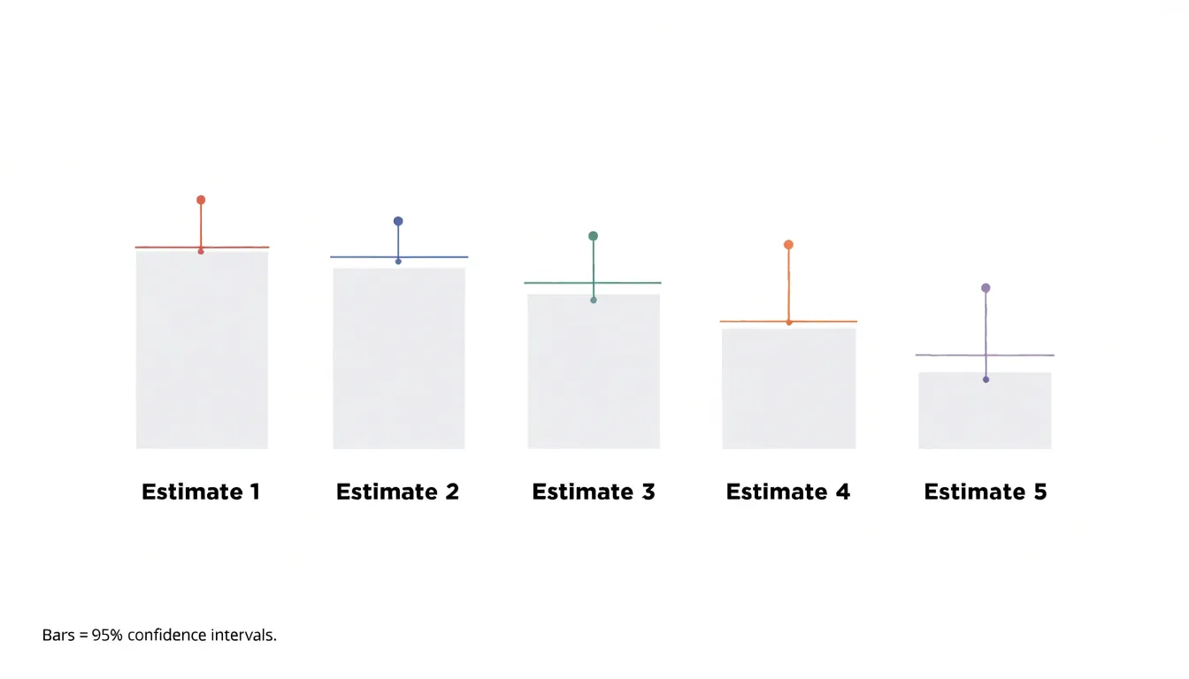
The underlying statistic behind an error bar matters, and charts usually rely on one of three conventions:
- Standard deviation bars show the spread of individual observations around the mean, useful when the goal is describing variability within a sample.
- Standard error bars shrink as sample size grows and reflect the precision of the estimated mean rather than the spread of raw values.
- Confidence intervals span a range that, under repeated sampling, would contain the true population value a stated proportion of the time, typically 95 percent. A confidence interval bar is therefore usually longer than a standard error bar and carries a clearer inferential meaning.
Traditional T-bars handle these distinctions well when labeled explicitly. A short caption or axis note identifying which statistic is shown prevents misreading, since the same visual length can imply very different things under different conventions.
Symmetric bars suit most distributions, while asymmetric bars can represent skewed confidence intervals or bounded ranges. Placing caps on both ends and keeping line weight light enough to avoid competing with the data points helps the bars read as annotation rather than a primary series. With consistent styling, error bars let viewers quickly grasp where precision is high, where estimates are shaky, and which comparisons between groups are worth trusting.
Confidence Bands
Confidence bands are a fundamental tool for visualizing uncertainty in time-series data, particularly when presenting forecasts or trend estimates. By adding a shaded region around a central trendline, they depict the range within which future observations are likely to fall, given the model’s assumptions. This shaded area is typically constructed using statistical techniques such as bootstrapping, Bayesian inference, or frequentist confidence intervals, which quantify the uncertainty inherent in the prediction. For example, a 95% confidence band indicates that, under repeated sampling, 95% of such bands would contain the true underlying trend.
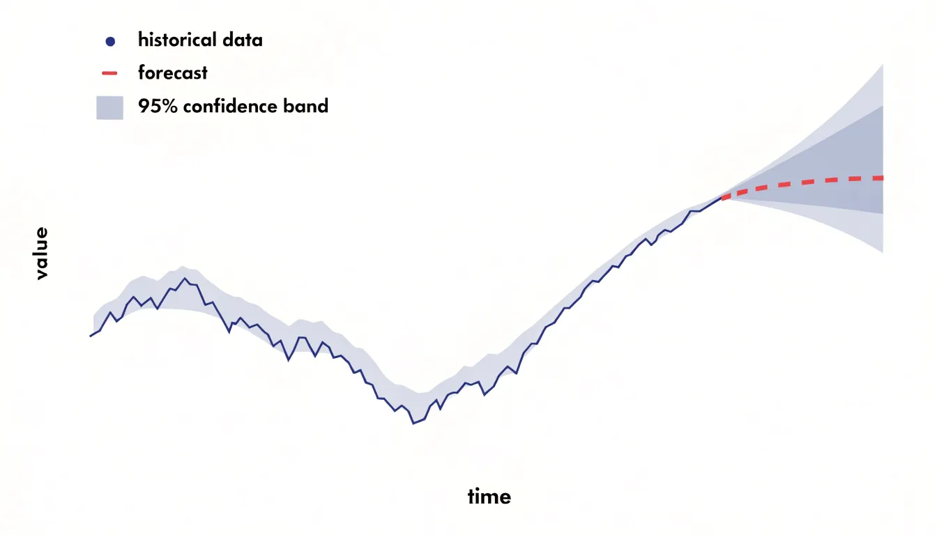
In practice, the band’s width varies along the x-axis, often widening as the forecast horizon extends to reflect increasing uncertainty. This visual cue helps viewers grasp that predictions become less reliable over time.
When designing confidence bands, choose an appropriate confidence level (e.g., 80%, 95%) and clearly label what the band represents. Using semi-transparent shading allows the underlying data points to remain visible, while a distinct border can delineate the band’s edges. It is also important to avoid implying that the band represents a hard boundary; rather, it is a probabilistic statement. Confidence bands differ from prediction intervals, which account for both model uncertainty and inherent randomness in the data, resulting in wider bands. Incorporating confidence bands into line graphs moves the display beyond a single deterministic line to a more honest representation of what is known and unknown.
Box Plots
Box plots provide a compact way to show the distribution of a numerical variable through five summary statistics: the minimum, first quartile, median, third quartile, and maximum. The central box spans the interquartile range, covering the middle fifty percent of observations, while a line inside the box marks the median. This arrangement lets a viewer compare the central tendency and spread of several groups at once, since the height of the box communicates variability directly and the median line reveals skew when it sits off-center.
Whiskers extend from the box to indicate the range of typical values, often reaching out to one and a half times the interquartile range beyond the quartiles. Points plotted past the whiskers flag observations that fall well outside the bulk of the data, drawing attention to values worth investigating—whether those are measurement errors, rare events, or genuinely important cases. Because the display relies on robust statistics, a handful of extreme values will not distort the box and median the way they would shift a mean, so the plot keeps its shape even when unusual observations appear.
Analysts can place several box plots side by side to compare treatments, time periods, or categories, and the alignment of whiskers and outlier markers across groups makes patterns of dispersion easy to read. Clear labeling of quartiles and outlier rules helps audiences interpret the plot correctly, and pairing it with sample sizes in the caption prevents viewers from over-reading narrow boxes built on few records.
Violin Plots
Violin plots combine kernel density estimation with box plot elements to show both the shape and spread of a distribution. The kernel density estimate produces a smooth curve that represents the probability density of the data at different values, while the box plot elements—typically a central line for the median and a thicker bar for the interquartile range—summarize central tendency and variability. This combination reveals features like skewness and multiple peaks, which are often obscured by standard summaries such as mean and standard deviation.
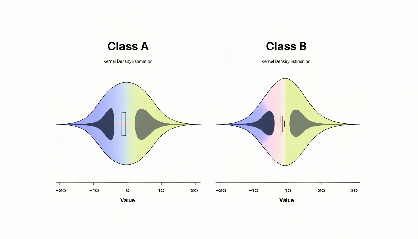
One of the key advantages of violin plots is their ability to reveal multimodal distributions. When data contain subgroups or clusters, the kernel density estimate shows multiple peaks, indicating distinct modes. For example, in a dataset of customer ages, a violin plot might show peaks around 25–34 and 45–54, suggesting two primary customer segments that traditional box plots or bar charts of averages would hide.
The width of the violin at each y-value (or x-value, depending on orientation) indicates the density of data points at that value. Wider sections represent a higher concentration of data, while narrower sections indicate fewer observations.
When using violin plots, consider the kernel density estimation parameters, such as bandwidth, as they can affect the plot’s appearance. A well-chosen bandwidth smooths out noise while preserving meaningful features. Violin plots are particularly effective for medium to large datasets, where density estimation is reliable; for small samples, the density estimate may be unstable and misleading.
Dot Plots
A dot plot places each observation as a single mark along a shared axis, so every data value has a visible counterpart on the page. When a dataset contains a dozen measurements or a few hundred, this one-to-one correspondence lets a reader count the marks and immediately grasp the sample size. Larger samples produce denser clusters of dots, while smaller samples leave visible gaps, and this density itself communicates how much evidence supports the summary statistics. The approach works especially well for small or moderate datasets, where aggregation into bars or bins would hide the fine structure of the data.
Because each dot sits at its exact recorded value, subtle variations remain visible. A dot plot can reveal a slight skew, a pair of outlying measurements, or a second cluster that a coarse histogram might smooth away. Stacking repeated values vertically, or using jitter for near-identical values, keeps individual observations distinguishable while still showing where the mass of the data lies. The reader can see both the overall shape and the granular detail in the same view.
The spread of the dots shows the range of variation, and the gaps between marks indicate how much the measurements differ from one another. Sparse regions of the plot remind the reader that estimates based on few observations carry more uncertainty than those supported by dense clusters. Marking summary statistics such as a median or mean alongside the raw dots gives context for how representative a central value is.
Dot plots work best when the axis is chosen to match the measurement scale and when marks are sized so that overlaps remain readable. With these adjustments, the plot becomes a compact, honest view of the underlying observations.
Heatmaps
Heatmaps translate numerical uncertainty into visual intensity, letting color highlight where risk concentrates across a spatial or tabular layout. A sequential gradient, running from pale tones to saturated ones, encodes probability or variance so that regions of high uncertainty draw the eye immediately. When a heatmap maps a city district, an image grid, or a matrix of estimates, the darkest cells reveal where confidence drops or where outcomes diverge most sharply from expectations.
Diverging palettes add a further layer, placing a neutral midpoint between two contrasting hues so viewers can see which side of a threshold a value falls on and how strongly it deviates. This makes heatmaps particularly effective for spotting clusters of statistical variance that tables of raw numbers would obscure. The visual density of color communicates magnitude without requiring the reader to parse each individual figure, which matters when decision-makers need to scan for problem areas quickly.
Analysts can pair the color field with annotations, such as marks on cells that exceed a variance threshold, to combine broad pattern recognition with precise callouts. Perceptually uniform and colorblind-safe palettes help avoid false boundaries and keep the encoding legible. A legend anchored to actual probability values grounds the visual impression in real quantities, while small-multiple heatmaps allow side-by-side comparison of uncertainty across scenarios or time periods.
Distribution Curves
Distribution curves show the full landscape of possible outcomes rather than a single point estimate. A bell curve, or normal distribution, places the most probable value at its peak and tapers symmetrically toward the extremes, giving viewers an immediate sense of where results are likely to cluster and how quickly certainty falls away from the center. The width of the curve matters as much as its peak: a narrow curve signals tightly grouped, predictable outcomes, while a wide curve shows that results could plausibly land across a broad range.
Probability density functions generalize this idea beyond the familiar bell shape to depict data that skews, clusters around multiple modes, or trails off unevenly. The height of the curve at any point reflects how likely values near that point are, so the area under the curve between two values corresponds to the probability of landing in that interval. This makes density plots especially useful for answering practical questions such as how often a metric might exceed a threshold or fall below a target.
The tails of these curves deserve particular attention when visualizing uncertainty. Extreme occurrences, though rare, often carry the greatest consequences, and a distribution curve makes their likelihood visible in a way that averages and summaries cannot. A long right tail, for instance, tells viewers that unusually large values are possible even if they are uncommon. Annotating tail regions with shaded areas or probability labels helps audiences understand the odds of worst-case or best-case scenarios. Overlaying distributions from different models, time periods, or groups further lets viewers compare expected values and the spread of risk side by side.
Ensemble Plots
Ensemble plots communicate uncertainty by showing multiple outcomes side by side rather than summarizing them into a single range or band. The technique involves plotting several simulation trajectories, model runs, or scenario paths on the same set of axes, letting viewers see how those paths fan out, converge, or diverge over time. Each line represents one plausible realization of the future, and the spread among the lines conveys the degree of uncertainty at any given point along the x-axis.
This works especially well for time series data where uncertainty compounds as forecasts extend further into the future. Weather forecasting offers the canonical example: meteorologists routinely run dozens of model perturbations from slightly different initial conditions and plot them together, producing the familiar spaghetti plot in which tight clustering near the present gives way to wide divergence days out. The same logic applies to financial scenario analysis, epidemiological projections, and climate modeling, where structural differences between scenarios matter as much as stochastic noise.
Ensemble plots are particularly effective at revealing structural scenario ranges—the distinct envelopes produced by different assumptions or model configurations rather than a single blended uncertainty band. When you overlay trajectories from multiple scenarios, viewers can see whether outcomes cluster into separate groups, whether some scenarios produce dramatically wider spreads than others, and where in time the divergence becomes meaningful.
A few design choices improve readability:
- Using transparency or thin lines to prevent overplotting.
- Coloring trajectories by scenario or model to make group membership legible.
- Highlighting a median or reference path without obscuring the individual runs.
The result is an honest, granular picture of forecast divergence that preserves the texture of individual outcomes rather than collapsing them into a summary statistic.
Animated Charts
Animated charts convey how probabilities shift over time by turning static numbers into motion that viewers can follow directly. Dynamic temporal visualizations show a probability distribution evolving frame by frame, so instead of reading a fixed interval, the audience watches the range widen, narrow, or drift as new information arrives. A forecast that begins with a broad spread of plausible outcomes can visibly tighten as the horizon shortens. This temporal dimension matters because many real-world quantities—from disease prevalence to stock returns to election margins—carry uncertainty that changes shape week by week, and a single snapshot can hide those changes entirely. By animating the distribution, the chart keeps the viewer oriented to how confidence builds or erodes over the observation period.
Hypothetical outcome plots (HOPs) extend this idea by displaying one plausible realization at a time, rapidly cycling through many draws from the underlying probability model. Each frame shows a single outcome: a dot, a bar, or a line at a concrete value. Across dozens of frames, the viewer sees individual possibilities flicker past and gradually forms an intuitive sense of which outcomes occur often and which are rare. The flicker frequency does the statistical work that a confidence interval would otherwise have to state explicitly.
This approach helps users who find abstract probability statements difficult to interpret, because the animation converts density into visible repetition. The method also supports temporal structure, since a HOP can show an entire trajectory sampled from a model and then replace it with another, letting viewers perceive both the path of a single scenario and the spread of scenarios across time. Used together, dynamic visualizations and HOPs let uncertainty be felt as fluctuating possibility rather than read as a fixed summary.
Icon Arrays
Icon arrays are grid-based pictographs in which each cell of a regular matrix stands for one person, one event, or one unit of risk. A common form is a ten-by-ten grid of one hundred icons, where filled symbols mark the people who experience an outcome and outlined or faded symbols mark those who do not. Because every cell carries the same meaning and the cells are arranged in a predictable order, a viewer can read the display by counting rather than by interpreting an axis, a scale, or a percentage. This makes icon arrays especially useful for communicating proportional risk and natural frequencies to audiences without statistical training.
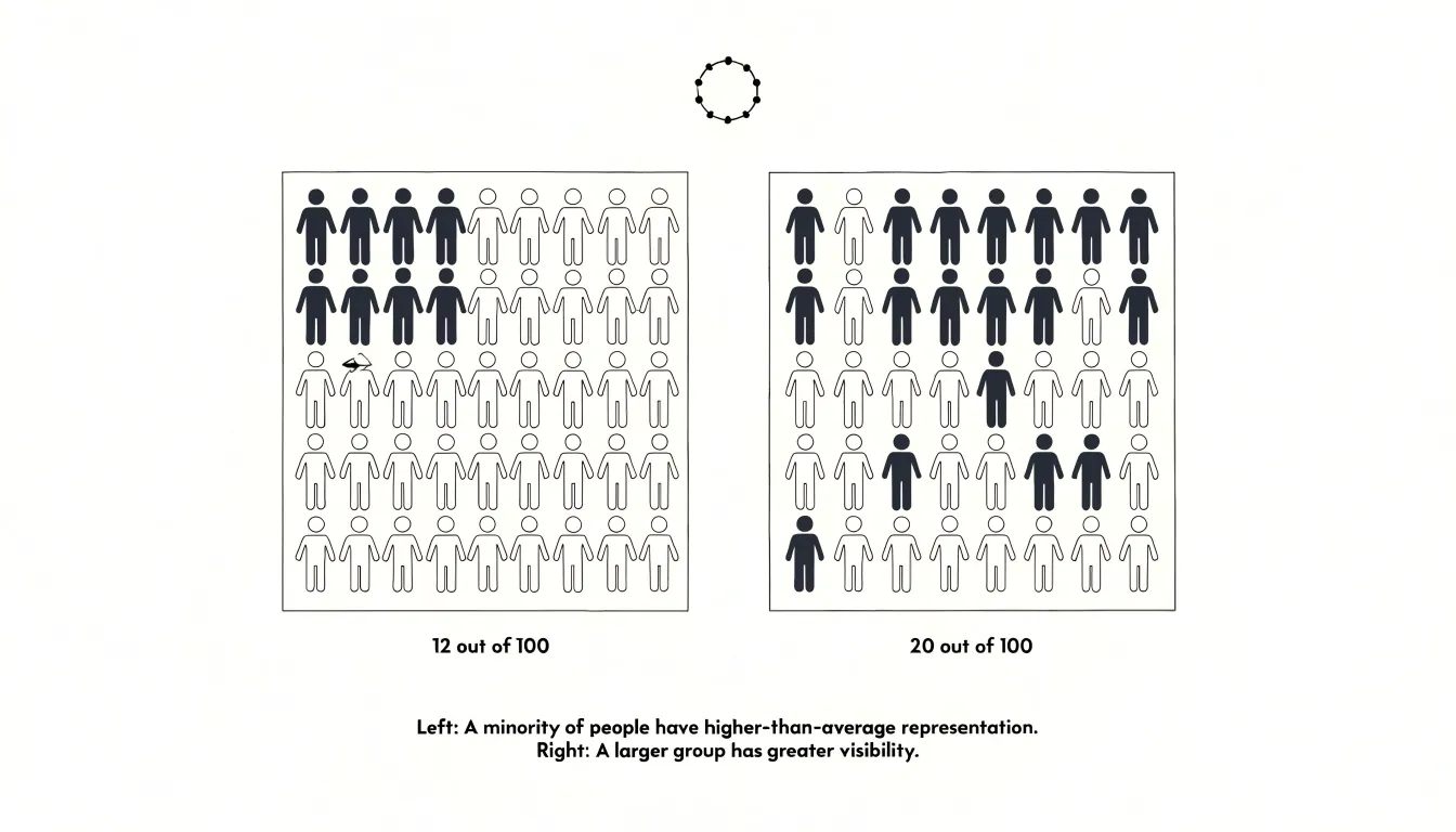
The design advantage lies in how directly the display maps onto the underlying quantities. Natural frequencies, such as “12 out of 100 people,” correspond to twelve filled icons in a grid of one hundred, so the risk appears as a visible cluster of marks that can be compared side by side with a second array. Viewers can see, for example, that one treatment group has noticeably more filled icons than another, or that the difference amounts to only a few cells. Ordering the filled icons in a block or grouping them in a corner reinforces this counting, while systematically grouping filled icons across arrays lets a viewer carry accumulated counts forward when comparing several outcomes.
Icon arrays also carry affective weight that abstract numbers often lack. A person represented by a filled icon reads as an individual, and a small cluster of filled icons conveys rarity in a way that a decimal probability rarely does. Designers can strengthen this by using a single humanoid shape rather than a generic dot, and by keeping the grid small enough to scan at a glance. The main caution is that the grid size must match the denominator being described, so that one icon always represents one case.
Common Pitfalls
Visualizations of uncertainty serve their purpose only when viewers interpret them as the designer intended, and a number of recurring design errors undermine that goal. Misleading scales rank among the most consequential. When an axis is truncated so that it begins above zero, small differences between values appear dramatic, and confidence intervals that are actually wide look tight and reassuring. A bar chart whose baseline has been shifted can make a modest estimate with substantial error bars resemble a precise, decisive finding. The practical safeguard is to inspect every axis deliberately, asking whether the range shown reflects the data honestly or has been cropped to heighten an effect.
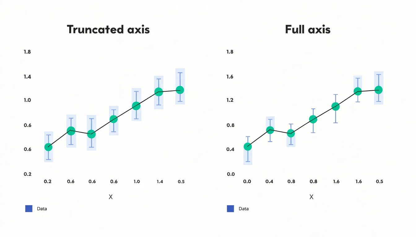
Truncated axes represent a specific instance of a broader problem: scales and encodings that distort perceived magnitude. Inconsistent units across panels, logarithmic axes presented without labeling, and area or bubble encodings that scale by radius rather than by area all cause viewers to misjudge the size of an effect relative to its uncertainty. These choices are often unintentional, arising from default settings in charting software, yet their impact on stakeholder decisions can be substantial.
Visual clutter presents a different failure mode. Layering shaded confidence bands, individual data points, trend lines, annotations, and multiple overlapping series into a single frame may technically display the uncertainty while functionally hiding it. When a chart requires extended study to locate the interval boundaries, the confidence information has effectively been buried. Reviewers should test whether the uncertainty band remains distinguishable at a glance when the chart is projected in a meeting or viewed on a small screen.
Avoiding these pitfalls requires disciplined review rather than sophisticated technique: check axis origins, verify that encodings map proportionally to the quantities they represent, and simplify until the confidence information stands out clearly.
Color Choices
When the goal is to communicate uncertainty, color choices need deliberate attention. The most reliable starting point is a perceptually uniform palette, one in which equal steps in data value produce equal steps in perceived color difference. Palettes such as viridis or the corresponding color maps in tools like ColorBrewer are designed with this property, so a value halfway along the scale looks halfway along the scale rather than bunching up in the greens or jumping abruptly in the yellows. Because the reader is judging gradations of confidence, a scale with uneven perceptual steps will make moderate uncertainty look either more or less severe than it actually is.
Opacity gradients offer a complementary approach, particularly for overlaid layers and probability bands. Rendering a wider uncertainty range with lower opacity lets the viewer see the distribution of possible values as a soft envelope around the central estimate, while a narrow range appears more solid and assertive. Varying transparency in this way maps naturally onto the everyday intuition that faint things are less definite than bold things. The technique does require care when multiple translucent layers overlap, since blending can create unintended colors and muddy the reading.
Accessibility deserves equal weight. Roughly one in twelve men has some form of color vision deficiency, and red-green scales in particular collapse for these readers, turning an informative gradient into an indistinguishable smear. Sequential palettes that vary in lightness as well as hue, and diverging palettes that avoid relying on red versus green alone, keep the uncertainty visible to everyone. Pairing color with a second cue—such as texture, contour lines, or labeled thresholds—provides redundancy so that the meaning survives even when hue perception does not. Testing the final graphic under simulated colorblindness is a quick and worthwhile check before publication.
Labels and Explanations
When a reader encounters a confidence interval, a p-value, or a standard deviation, the chart itself should carry enough plain-language context for that reader to understand what the numbers mean without consulting a statistics textbook. The work begins with annotations placed directly on or beside the relevant visual element, so the explanation sits where the reader’s eye already is. A shaded band can be labeled simply as a range within which the true value is likely to fall, with the specific percentage spelled out. A spike in a trend line can carry a short note describing what happened and why it matters.
Captions extend this work by summarizing the chart’s central message in a sentence or two, giving readers a frame before they interpret the details. Microcopy handles the smaller elements: axis labels, legend entries, and tooltips each offer a moment to replace jargon with direct language:
- A standard deviation might become “a typical distance from the average.”
- A p-value might become “the chance of seeing a result this extreme if there were really no effect.”
Plain language does not mean vague language; it means choosing words that carry the same meaning for a general audience that the technical term carries for a specialist. Consistent phrasing across a chart or a whole report helps readers build familiarity as they move from one visual to the next. Reviewing drafts with someone outside the analytical team is a practical way to catch terms that still assume too much.
Interactive Tools
Interactive tools turn static uncertainty visualizations into exploratory environments where users can test assumptions and see immediate consequences. Sliders allow users to adjust key parameters—such as confidence levels, forecast horizons, or model weights—and watch how the displayed uncertainty changes in real time. This hands-on manipulation helps users build intuition for how sensitive a model is to different inputs, and it lets them align the visualization with their own beliefs or decision criteria.
Hover states add another layer of exploration by revealing detailed information on demand. When a user hovers over a data point or a region of a distribution, tooltips can display exact values, credible intervals, or the underlying data that produced the estimate. This keeps the main view uncluttered while providing depth for those who seek it.
Parameter controls go further, enabling users to switch between different uncertainty representations or to adjust the scale of the visualization. For example, a control might let users toggle between absolute and relative uncertainty, or between different probability thresholds. By empowering users to personalize the uncertainty model, these tools let them explore scenarios that matter to them, compare outcomes, and understand the risks and trade-offs involved.
Dashboards
Dashboards offer a natural home for uncertainty visualization because they gather multiple views of a dataset into a single surface. Integrating uncertainty displays into that surface means each panel communicates not just a central estimate, but the range of plausible outcomes around it. A trend line paired with a shaded confidence band, a forecast chart with fanning intervals, or a map with graduated uncertainty overlays all convey risk in ways suited to different questions, giving decision-makers a layered reading that no single chart could provide on its own.
The design challenge lies in combining complementary formats so they reinforce one another rather than compete for attention. A summary metric tile can show a headline figure with a compact interval marker, while the larger panel beneath it breaks that figure into fan charts or distribution strips. A heatmap can carry a secondary overlay that flags where estimates are least reliable. Consistency across panels matters: shared color scales for uncertainty magnitude, aligned time horizons, and matching confidence levels let viewers compare panels without reinterpreting each one. When these conventions hold steady, the dashboard reads as a single coherent narrative about risk rather than a patchwork of unrelated charts.
This integration supports multi-layered decision-making. Executives can move from a high-level view of overall uncertainty down to specific dimensions where variability is concentrated, then back out to weigh trade-offs across the whole picture. Planning discussions shift from debating single numbers toward reasoning about ranges and probabilities, which grounds strategic choices in realistic expectations. A well-composed uncertainty dashboard turns ambiguity from a source of hesitation into structured information that teams can examine, compare, and act on with greater confidence.
Frequently Asked Questions
What do error bars show on a chart?
Error bars communicate the range within which a value is likely to fall, and the length of the bar signals the magnitude of uncertainty. A short bar suggests a tightly measured value, while a long bar warns viewers to treat the point estimate with caution.
How do confidence bands show uncertainty in forecasts?
Confidence bands add a shaded region around a central trendline to depict the range within which future observations are likely to fall, given the model’s assumptions. The band’s width often varies along the x-axis and can widen as the forecast horizon extends to reflect increasing uncertainty.
What do box plots show?
Box plots show the distribution of a numerical variable through five summary statistics: the minimum, first quartile, median, third quartile, and maximum. The central box spans the interquartile range, covering the middle fifty percent of observations, while whiskers indicate the range of typical values and points past the whiskers flag outliers.
When are violin plots not appropriate?
Violin plots are particularly effective for medium to large datasets, where density estimation is reliable. For small samples, the density estimate may be unstable and misleading.
Why should I avoid truncated axes in uncertainty charts?
When an axis is truncated so that it begins above zero, small differences between values appear dramatic, and confidence intervals that are actually wide can look tight and reassuring. The article recommends inspecting every axis deliberately to see whether the range shown reflects the data honestly.
How can I make color choices accessible for uncertainty visualizations?
Use perceptually uniform and colorblind-safe palettes, because roughly one in twelve men has some form of color vision deficiency and red-green scales in particular can collapse for these readers. Sequential palettes that vary in lightness as well as hue, diverging palettes that avoid relying on red versus green alone, and a second cue such as texture, contour lines, or labeled thresholds help keep uncertainty visible. Testing the final graphic under simulated colorblindness is recommended before publication.
Tony Astor
Tony writes about data visualization and the tools people use to build charts and dashboards. More about Data Illustrator