How to Visualize Small Datasets Effectively
 By Tony Astor ·
How to Visualize Small Datasets Effectively
Use a dot plot for small datasets: each observation appears as one mark, stacked where values repeat, so every raw data point stays visible without binning or averaging. It suits up to roughly 20–30 observations and reveals spread, gaps, ties, and outliers directly, unlike histograms or box plots that hide individual values.
Table of Contents
Dot Plots
A dot plot displays each observation in a dataset as a single mark, usually placed above a shared horizontal axis. When several values coincide, the marks stack vertically, producing a column whose height shows how often that value occurs. Because no step in constructing the plot combines, averages, or bins the measurements, every original data point remains visible on the chart. A reader can count the marks and recover the underlying values, which gives the display a transparency that summary statistics alone cannot offer. For small sample sizes, this transparency matters a great deal; with only a dozen or two observations, each measurement carries real weight, and losing any of them to aggregation can distort the picture.
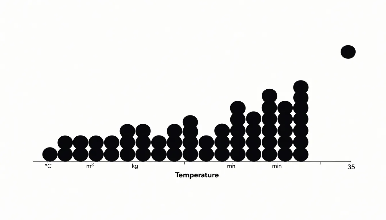
Small datasets are especially vulnerable to the distortions introduced by grouping. Histograms divide a range into bins, and the choice of bin width can make the same data look clustered or spread out. Box plots reduce a distribution to five summary numbers and hide the shape between the quartiles. A dot plot sidesteps these issues by presenting the raw record directly. Outliers appear as isolated marks rather than being absorbed into a bin. Ties are explicit, since stacked dots show exactly how many observations share a value.
A dot plot works well with sample sizes up to roughly twenty or thirty observations, at which point the stacks can become tall and the display crowded. Jittering or using a strip plot can extend the range slightly. Labeling the axis with meaningful units and choosing sensible spacing between values keeps the plot legible. The finished chart answers questions about spread, shape, gaps, and repeated values in a single view, which makes it a dependable first choice for exploratory work on small samples.
Bar Charts
Bar charts compare discrete categories through a simple visual contract: the length of each bar maps directly to a value. To honor that contract, start with a clean baseline at zero. Truncating the axis exaggerates differences and invites misreading, so keep the scale honest and let the bar lengths carry the comparison. When categories have long or numerous labels, a horizontal layout usually reads better, since text stays upright and doesn’t collide with neighboring bars. Reserve vertical bars for short labels or time-based sequences where the left-to-right reading order feels natural.
Order the bars purposefully. Sorting by value rather than alphabetically turns the chart into an instant ranking and helps viewers spot the largest and smallest entries without scanning back and forth. If the categories have an inherent order, such as age brackets, preserve that sequence instead. Keep color meaningful rather than decorative: a single uniform fill works well for most comparisons, with a highlight reserved for the category you want to emphasize. Limit the number of bars; beyond roughly a dozen, consider grouping, filtering, or switching to a different form.
Give bars a consistent width and spacing, and leave modest gaps between groups if you use clustered bars. Omit or lighten gridlines when value labels are shown directly, keep tick marks minimal, and avoid three-dimensional effects, shadows, and patterns that distort how length is perceived. Label axes clearly with units, add a concise title that states the takeaway, and annotate notable values directly on the chart when space allows.
Strip Plots
A strip plot places every data point as an individual mark along a single axis, grouping points by category when sub-groups exist. When you arrange points side by side for each sub-group, the plot becomes a compact visual summary of where values fall and how they cluster without losing raw values to binning or summary statistics.
You can see the full range, the spread, and the shape of each sub-group at a glance. Gaps between points indicate sparse regions, while dense clusters show where most values concentrate. This is especially useful when the dataset is too small for a histogram or box plot to estimate density or quartiles reliably.
Overlaps across sub-groups also become apparent. When points from different categories share the same region of the axis, their positions may coincide or nearly coincide. Adding a small amount of horizontal jitter separates overlapping marks without altering their vertical positions, making it clear which points belong to which group while maintaining the integrity of the values.
Because every value remains visible, you can spot outliers, identify multimodal patterns, and observe whether sub-groups have similar centers, spreads, or shapes. This level of detail supports both exploratory analysis and communicating findings to an audience that may want to verify the raw data.
Line Graphs
Line graphs are a natural fit for brief time-series data, such as a week of daily sales figures, a month of weekly heartbeat readings, or hourly temperatures across a single afternoon. Begin by plotting each recorded value as a marker at its true position and connecting the points in chronological order, which preserves the actual sequence of events. When datasets are this small, showing individual markers alongside the line helps readers see exactly where measurements were taken and prevents the line from implying continuous data between readings that may not exist.
Axis scale management is where small line graphs succeed or fail. Default scales often span zero to the maximum value, compressing a series that ranges between 68 and 74 degrees into a nearly flat line. Where minor fluctuations are the story, narrowing the vertical axis to a range that brackets the observed values, with a little padding above and below, makes short-term movement visible. Label the axis clearly so readers know the scale has been adjusted, and state the chosen range in the chart subtitle or caption. A grid or horizontal reference lines at regular intervals keep the reader oriented within the narrowed range.
Consistency across related charts matters as well. If several short series appear side by side, use the same vertical range for each so comparison stays fair. Keep the horizontal axis evenly spaced by time interval, and avoid gathering too many series onto one small chart, since overlapping lines quickly become unreadable.
Sparklines
Sparklines are compact, word-sized charts that sit directly inside a line of text or within a table cell, showing the shape of a trend across a series of values without the axes, labels, and gridlines of a conventional chart. In a dense report or dashboard, a single number such as a monthly total or a current balance tells the reader almost nothing about direction or volatility. Placing a small trendline next to that number lets the reader see at a glance whether a figure has climbed steadily, dipped sharply, or oscillated, while still reading the exact value it summarizes.
With only a dozen or so observations, the overall shape of the series is fully visible in a sparkline, and subtle features such as a mid-period plateau or a late upturn remain legible rather than collapsing into noise. The inline format also keeps the reader’s eye moving through the report: each row stays self-contained, with the value and its trend sitting side by side, so comparisons across rows happen naturally without jumping to a separate chart area.
Sparklines can share a common scale or be scaled independently so that each row highlights its own trajectory. A reference line for an average or target adds a quiet benchmark, and color can flag the most recent value or the direction of change. In practice, sparklines are often accompanied by a brief caption to clarify what period or unit the trend covers, particularly when many rows appear together.
Before and After Charts
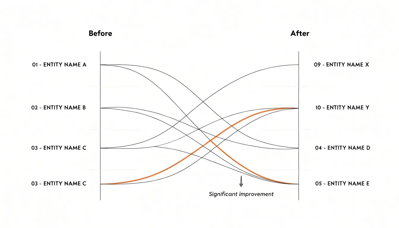
Before and after charts answer a specific question that aggregated statistics cannot: what happened to each individual between two points in time? When every row represents a person, team, or case that deserves to be seen on its own, paired change metrics are best shown by directly connecting the starting value to the ending value.
The slope chart is the classic form. Each entity gets a line running from its position in the first period to its position in the second, with lines allowed to cross freely. Those crossings are the point. A steep upward slope reads instantly as a large gain, a flat line shows little movement, and a downward slope flags a decline, all without a legend or a table of deltas. Placing the two time points as labeled columns on the left and right makes the ordering of change visible at a glance, especially when values are ranked at each endpoint.
The dumbbell plot applies the same logic horizontally. A dot marks the before value, another dot marks the after value, and a connecting bar shows the gap between them. With the categories listed down the y-axis, the length of each bar communicates the magnitude of change, and the direction tells you whether the shift was positive or negative. Dumbbell plots handle longer category labels gracefully and make the size of the gap easy to compare across rows.
Both formats keep the individual visible, which matters when one dramatic transition would otherwise be buried inside an average. Annotating a few notable cases with names or short labels turns the chart from a summary into a record of who moved and by how much.
Grouped Charts
Grouped charts place two series next to each other within the same category slot, which makes them a natural fit for small-cohort comparisons. Start by deciding which dimension belongs on the category axis: usually this is the cohort, condition, or time point, while the two groups being compared become the paired marks within each category. Each pair should sit close together, with a wider gap separating neighboring categories so the eye reads pair-then-pair rather than an undifferentiated row of bars.
Side-by-side bars work well when values represent counts or totals and the bars share a common baseline. Keep the bars slender and the paired spacing tight; thick bars with narrow gaps turn a twelve-value chart into a solid block. Dot plots handle the same comparison with less ink, and they shine when the values are means with ranges or individual observations. A dot plot can show one marker per group along a shared horizontal scale, joined by a thin connector line that makes the gap between the two groups the visual focus.
With only two groups, skip the legend entirely and label the series directly using short headers above each column pair, or place a single compact key at the top-left of the plot area. Color should carry the group identity consistently, using two hues that remain distinguishable in grayscale and for color-blind readers. One reference line at zero or at a meaningful target, plain axis labels, and direct group labels are enough to make the size and direction of the difference obvious.
Color Highlighting
Selective accent colors act as visual signposts, guiding the reader’s eye to the most important insights while allowing secondary elements to recede. Choose a single, saturated hue for the data you want to emphasize—perhaps the peak sales month, the outlier in a scatter plot, or the category that exceeds a target—and render all other elements in muted grays or desaturated tones. This contrast creates an immediate hierarchy. For example, in a line chart tracking monthly revenue, you might color the line gray but highlight the month with the highest growth in a bold orange. Because human vision is highly sensitive to color contrast, a single pop of color against a neutral background stands out without requiring extra labels.
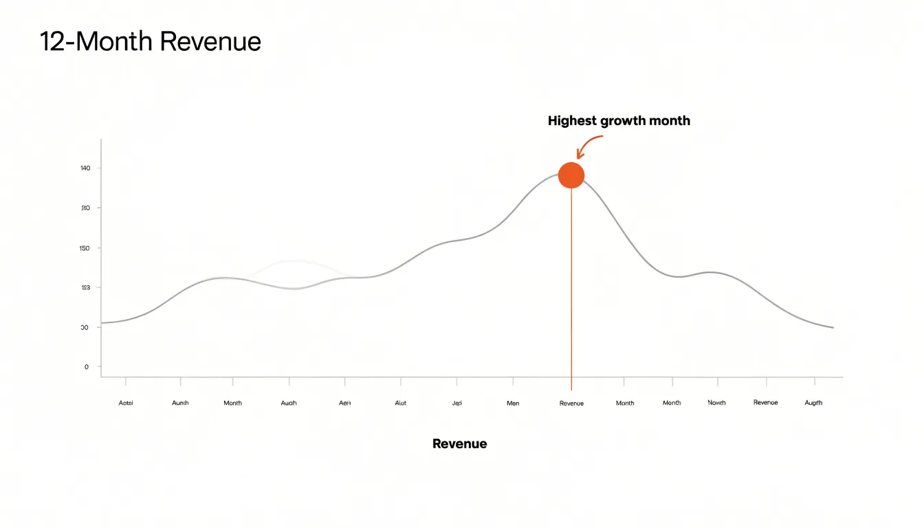
When applying color highlighting, use the same accent color for all elements that share the same meaning, and avoid using multiple accent colors unless they represent distinct categories. Choose colorblind-friendly palettes, such as blue-orange combinations, to ensure accessibility.
Sorting
When a chart of a small dataset is sorted by magnitude, the ordering itself carries information. Alphabetical sorting is a filing convention; it answers the question of where a value sits in a list rather than how it compares to its neighbors. Ordering values from largest to smallest lets a reader’s eye travel down the chart in the same direction as the underlying measure, making rank legible at a glance. The top performer appears at the edge of the chart where attention naturally lands first, and the distance between the leader and the next entry registers instantly. Extreme values stand out on their own rather than being buried in an arbitrary position, so outliers and anomalies announce themselves without requiring the reader to compare every bar against every other.
In a bar chart, sorting by magnitude produces a monotonic descending or ascending staircase that makes relative proportion easy to read, while an alphabetical arrangement creates a jagged profile that requires mental reordering to interpret. The same principle applies to dot plots and lollipop charts. Grouping tied or near-tied values with magnitude sorting also reveals clusters and gaps that might otherwise stay hidden. For a report audience scanning a small chart in a few seconds, this ordering states rank, notable high and low points, and the overall shape of the distribution immediately.
Data Labels
Unlike axes that require mental mapping and estimation, data labels place the exact value right next to the data mark, allowing audience members to read figures at a glance. This is especially useful when the chart contains only a handful of points and individual values matter more than overall trends.
Use data labels when the exact number is the key message. In a bar chart comparing quarterly revenue across four regions, labeling each bar with its dollar amount eliminates guesswork. Similarly, in a line chart with five time points, labels on each marker clarify the trajectory without forcing readers to trace back to the y-axis. When axes are cluttered with fine gridlines or when the scale is non-linear, labels provide direct clarity.
Place labels near the data point, typically above bars or beside markers, with enough contrast to stand out without competing with the data itself. Avoid overlapping labels by adjusting positions or using callouts. For very small datasets, you can remove the y-axis entirely and rely solely on labels to convey values, reducing visual clutter and focusing attention on the numbers.
Direct Annotations
Direct annotations place explanatory text right beside the data point it describes. When a line chart shows a sudden spike or a bar dips well below its neighbors, a short callout attached to that point can say what happened: a product launch, a holiday closure, a data-entry correction, or a one-off event. Readers meet the explanation at the exact moment they wonder why the shape changed.
In a table of twelve monthly figures, one anomalous month can dominate the visual impression and shape how readers interpret the whole trend. Without context, that single point invites guesswork or dismissal. Leaving outliers unlabeled and describing them in surrounding paragraphs asks readers to hold the chart in memory while scanning for a matching sentence, and many will skip that step entirely. Placing the note on the chart resolves the question on the spot.
Keep the callout compact—a phrase or single sentence—positioned close enough that its connection to the point is unambiguous, with a thin leader line when spacing is tight. Match the tone of the surrounding labels and choose a color that separates the note from the plotted data while staying within the palette. Used sparingly, perhaps one or two annotations per chart, direct labeling turns an unexplained anomaly into a deliberate part of the narrative.
Tables With Visuals
A plain table of numbers asks the reader to scan across rows and columns to find the largest value or spot a trend. For small datasets, where every row is visible at once, a micro-bar chart placed beside each value turns the table into a dual-purpose tool. The number stays in place for precise lookups, while the bar length gives an immediate sense of relative size. A reader can scan the column of bars to see which category dominates, then read the exact figure when precision matters.
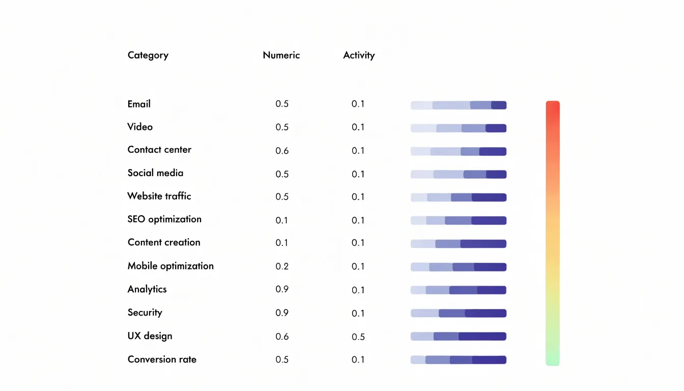
Heatmaps work the same way at the cell level. Shading each cell according to its value, from light to dark, lets patterns emerge from the grid itself. Highs and lows become immediately visible, and clusters of similar values show up as bands of consistent color. This is especially useful when a table has several numeric columns, since the shading draws the eye to the strongest and weakest entries without requiring a careful read of every cell. In a table with a dozen or two rows, a small bar or a color fill takes up little space and never overwhelms the text.
In most spreadsheet and reporting tools, a bar can be drawn with a simple formula using repeated characters or with built-in chart features, while conditional formatting handles heatmap shading automatically. Keep the visuals quiet and subordinate to the numbers, using consistent scales and restrained colors so the figures provide accuracy and the graphics provide orientation.
Decluttering
With only a handful of data points, extraneous features can easily overpower the information you are trying to convey. Removing unnecessary gridlines, redundant borders, and decorative elements allows the actual data points to become the primary visual focus.
Gridlines are often included by default in charting tools, but in a small chart where each point is clearly discernible, the axes or direct labels provide enough context for reading values. Similarly, redundant borders—such as boxes around the chart area, legend, or individual elements—add visual weight without adding meaning. Decorative elements like background fills, shadows, or 3D effects distract from the data and distort perception. Stripping away these non-essential elements gives the chart room to breathe and draws attention immediately to the relationships between points.
Mobile-Friendly Charts
A compact chart that looks crisp on a desktop monitor can collapse into an unreadable cluster of overlapping labels and hairline strokes on a smartphone. Rather than scaling a wide landscape chart down to fit a narrow viewport, design with a tall, narrow aspect ratio in mind or allow the chart to reflow so that axes and labels retain breathing room. Fixed pixel widths should give way to relative units so the chart can adapt to whatever space the device provides.
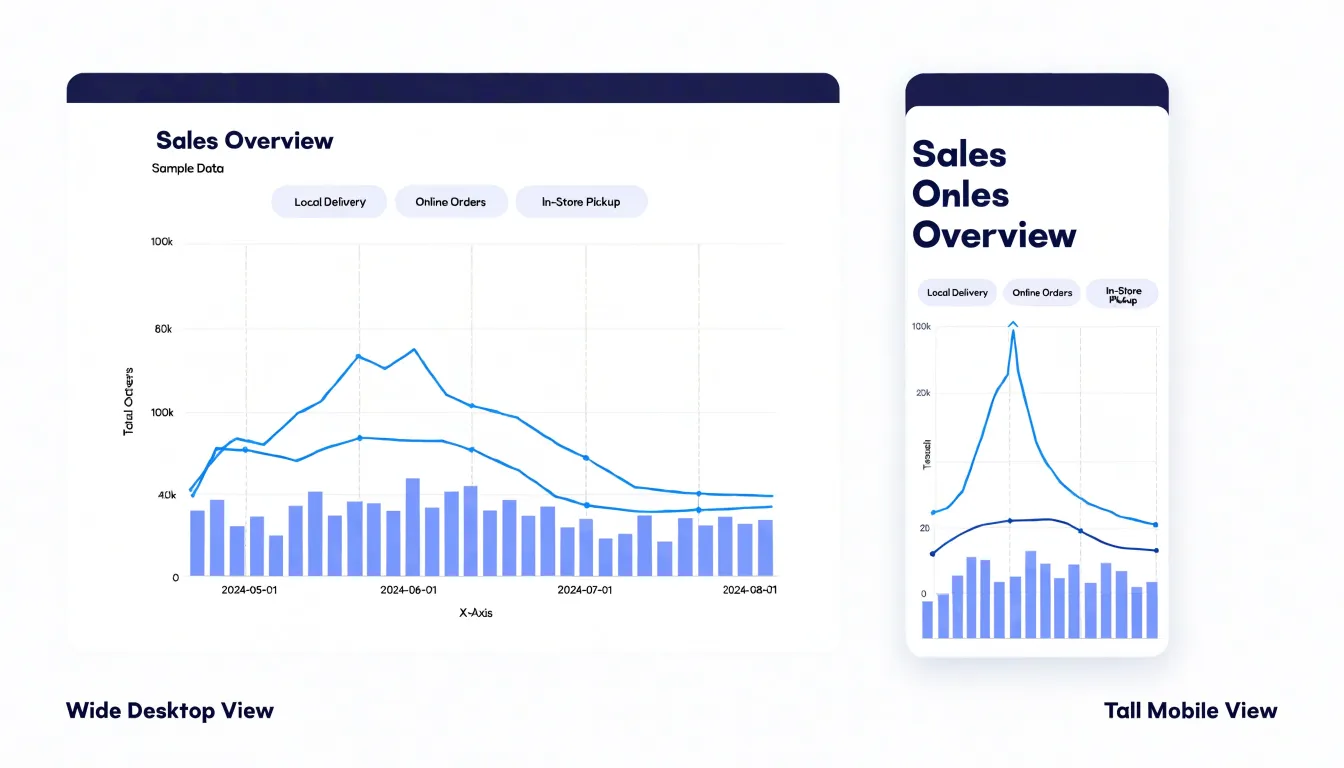
Font sizes deserve particular attention because text that sits comfortably at desktop scale becomes microscopic on a phone. Set labels, axis ticks, and legends at sizes that remain readable without zooming, and trim secondary text such as gridline annotations or move it into tooltips. Limiting the number of visible labels through sensible tick intervals keeps the chart clean while preserving meaning.
On a touchscreen, fingers are far less precise than a mouse pointer, so interactive elements such as data points, tooltip triggers, and legend toggles need generous hit areas. Spacing these elements apart prevents accidental taps and makes the chart feel responsive rather than fiddly.
Final Quality Check
Before a visualization is published, a structured review process catches problems that are easy to miss during creation.
- Verify data accuracy. Return to the source dataset and spot-check individual values against what appears in the chart. Confirm that totals add up, axis scales are consistent, and labels match the categories they describe. Recalculate any derived percentages or averages independently to rule out formula errors. Confirm that no truncated axis exaggerates differences and that units are stated clearly.
- Evaluate color contrast and accessibility. Test foreground and background color combinations against WCAG contrast ratios, aiming for at least 4.5:1 for body text and 3:1 for larger text and graphical elements, using a contrast checker tool rather than visual judgment. Simulate color blindness using a palette or browser plugin to ensure distinctions carried by color alone remain readable; add patterns, direct labels, or shape differences where they do not.
- Assess legibility across devices. View the visualization on a phone, tablet, and desktop screen, and at browser zoom levels of 150 and 200 percent. Check that text does not overlap, tick labels remain readable, and interactive elements have touch targets large enough for fingers. Print a grayscale copy to confirm that the chart survives without color.
- Complete a consistency pass. Verify titles, captions, and footnotes against the final data, confirm source attributions are present, and have a colleague review the chart with fresh eyes. Document each check and its outcome so the process is repeatable for future publications.
Frequently Asked Questions
How many data points can a dot plot handle?
A dot plot displays each observation as a single mark and stacks marks when values coincide, so every original data point remains visible. It works well with sample sizes up to roughly twenty or thirty observations; beyond that the stacks can become tall and crowded, though jittering or a strip plot can extend the range slightly.
Should a bar chart axis always start at zero?
Yes—bar charts should start with a clean baseline at zero. Truncating the axis exaggerates differences and invites misreading.
How can I show small fluctuations in a line graph?
For a series with only minor fluctuations, narrow the vertical axis to a range that brackets the observed values with a little padding above and below. Label the axis clearly, state the chosen range in the subtitle or caption, and use a grid or horizontal reference lines to keep readers oriented.
What is the difference between a slope chart and a dumbbell plot?
A slope chart gives each entity a line from its position in the first period to its position in the second, and crossings are allowed and can be the point. A dumbbell plot applies the same before-and-after logic horizontally, using two dots and a connecting bar so the gap’s length and direction are visible.
How do I use color highlighting without harming accessibility?
Choose a single saturated hue for the data you want to emphasize and render other elements in muted grays or desaturated tones, keeping the same accent color for elements with the same meaning. Avoid multiple accent colors unless they represent distinct categories, and choose colorblind-friendly palettes such as blue-orange combinations.
What contrast ratio should data visualization text meet?
Test foreground and background combinations against WCAG contrast ratios, aiming for at least 4.5:1 for body text and 3:1 for larger text and graphical elements. Use a contrast checker rather than visual judgment, and simulate color blindness to confirm distinctions carried by color alone remain readable.
Tony Astor
Tony writes about data visualization and the tools people use to build charts and dashboards. More about Data Illustrator