How to Visualize Relationships Between Variables
 By Tony Astor ·

How to Visualize Relationships Between Variables
Scatter plots show relationships between two continuous variables by plotting each observation as a point, where upward trends indicate positive correlation and downward trends indicate negative correlation; tight clusters signal strong association and outliers reveal anomalies. Line graphs track change over time, grouped bar charts compare categories, heat maps display correlation matrices, and box plots summarize distributions.
Table of Contents
Scatter Plots
Scatter plots map two continuous numerical variables side by side, assigning one to the horizontal axis and the other to the vertical axis. Each point represents a single observation, making this chart type effective for comparing pairs like height and weight, temperature and energy consumption, or advertising spend and sales revenue.
The overall pattern of the cloud reveals how the variables are associated:
- Positive correlation: Points trend upward from left to right, meaning higher values on one axis tend to accompany higher values on the other.
- Negative correlation: Points trend downward from left to right, meaning higher values on one axis tend to accompany lower values on the other.
- Strength of association: A tight band following a clear line or curve indicates a strong relationship, while a diffuse cloud indicates a weak one.
Scatter plots also expose features that summary statistics like correlation coefficients collapse into a single number. Tight clusters of points may indicate distinct subgroups, such as different customer types or experimental conditions. Points that fall far from the main cloud make outliers immediately visible. By showing raw observations, scatter plots provide an honest view of non-linear patterns, varying spread, and multiple modes, helping analysts generate hypotheses about underlying mechanisms.
Line Graphs
Line graphs track how variables change across a continuous span of time. Each point represents a measurement taken at a specific moment along an ordered horizontal timeline, and the line connecting them reveals rises, falls, plateaus, acceleration, and turning points.
Line graphs excel at surfacing two major temporal patterns:
- Seasonal fluctuations: When data is collected at regular intervals over months or years, recurring peaks and valleys often emerge—such as retail sales climbing during holidays or energy consumption rising in winter. A continuous timeline lets analysts separate predictable seasonal rhythms from unusual anomalies.
- Long-term directional shifts: A gradual upward slope across years signals sustained growth, while a downward drift points to persistent decline. These broad trends are hard to spot in raw number tables but immediately apparent as a line.
Plotting multiple lines on the same axes compares several metrics or categories simultaneously, showing whether trends move in parallel, diverge, or intersect.
Grouped Bar Charts
Grouped bar charts organize bars into clusters along a shared scale. Each cluster represents a discrete category (such as a region or demographic segment), and each bar within the cluster corresponds to a separate metric or subcategory (such as a specific year or survey response). Viewers can compare values both within a group and across groups by tracing bars in the same position and color from cluster to cluster.
For accurate side-by-side evaluation, keep the internal bar order, color coding, axis scales, and quantitative units identical across all clusters. Several design choices keep the chart readable:
- Limit cluster size: Restrict each cluster to three to five bars so the group does not become crowded.
- Order categories meaningfully: Arrange clusters by descending total value or a natural progression rather than arbitrarily.
- Set clear spacing: Keep gaps within a cluster tight and gaps between clusters wider so the grouping is visually obvious.
- Supplement color: Pair uniform metric colors with direct value annotations, labels, or patterns to support accessibility and reduce reliance on gridlines.
Heat Maps
Heat maps turn a two-dimensional grid of numbers into an instantly readable image by assigning each cell a color from a gradient. Because the brain processes color pre-attentively, bands and blocks of similar shade stand out before deliberate analysis begins.
This structure is particularly effective for multi-variable correlation matrices, where dozens of pairwise relationships sit side by side, and for performance tables laid out by time on one axis and category on the other. In a sequential gradient running from pale yellow through orange to deep red, the darkest cells mark the highest-density areas or strongest signals:
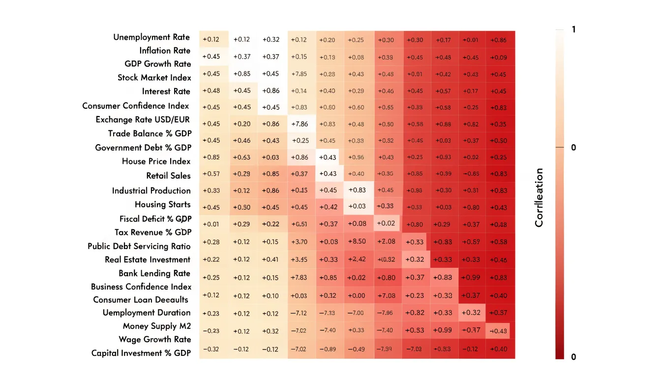
- Horizontal bands of dark cells indicate a category that scores high across every period.
- Vertical streaks highlight a single time point that affects all categories at once.
- Isolated dark cells draw attention to specific combinations worth investigating.
Match the color scale to the data’s structure: use a sequential gradient for values that increase in one direction, and a diverging gradient when values fall on either side of a meaningful midpoint (such as zero in a correlation matrix). Annotate cells with their raw values or provide a legend with explicit thresholds so viewers can read exact figures when needed.
Bubble Charts
A bubble chart extends a standard two-dimensional scatter plot by turning each point into a circle whose size encodes a third numerical variable. Adding a sequential or diverging color scale introduces a fourth dimension, allowing readers to compare rankings across multiple measures, spot gradients, and identify outliers in a single view.
Scale each circle’s area—not its radius or diameter—to the underlying value. Human vision judges circle size by area, so scaling by radius makes small values look disproportionately tiny and exaggerates large ones.
Because bubbles take up more space than simple points, crowded regions often suffer from occlusion. Keep overlapping markers legible by using transparent fills, subtle outlines, and restrained color palettes. Include clear legends for both size and color, and add interactive tooltips when viewers need exact values.
Box Plots
Box plots summarize a distribution using five statistics: the minimum, first quartile, median, third quartile, and maximum. Placing several box plots side by side along a shared axis allows quick comparison of center, spread, and skew across categories.
The box spans the first to third quartiles, capturing the middle 50 percent of the data (the interquartile range, or IQR). A tall box signals wide spread among typical observations; a short box indicates tight clustering. The line inside the box marks the median. When the median sits near the center and the whiskers extend roughly equal distances, the distribution is symmetric. When the median sits near one edge and one whisker stretches much farther, the distribution is skewed toward the longer whisker.
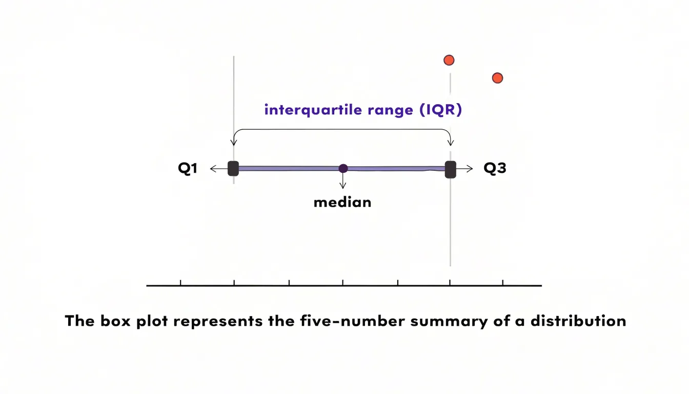
Points falling beyond the whiskers—typically defined as more than 1.5 times the IQR from the quartiles—are plotted as individual markers. This isolates extreme values without obscuring the main distribution.
Correlation and Causation
A correlation coefficient summarizes how closely two variables move together: values near 1 indicate they rise and fall in step, values near -1 indicate they move in opposite directions, and values near 0 suggest little linear relationship. However, co-occurrence does not prove that one variable changes the other. A third confounding factor may drive both variables, causality may run in the reverse direction, or the pattern may hold only within a specific subgroup or time window. For example, seasonal demand and staffing levels rise together, but both respond to the calendar rather than one directly causing the other.
When presenting correlated data to decision makers, separate what the data show from claims about the underlying mechanism:
- Pair scatter plots with trend lines and annotations that describe direction, strength, and outliers without overstating the conclusion.
- Use accurate language: Choose phrases like associated with, linked to, and tends to accompany rather than drives, causes, or leads to.
- State what is missing: Note unmeasured variables and outline the evidence needed to test causality, such as controlled experiments, natural experiments, longitudinal designs, or adjustments for confounders.
Outlier Spotting Techniques
Different chart types reveal unusual observations in distinct ways:
- Scatter plots: Points sitting far from the main cluster or fitted trend line.
- Box plots: Individual markers plotted beyond the 1.5 IQR whiskers.
- Histograms and density plots: Thin, isolated tails far from the central mass.
- Line charts: Sudden spikes or drops that break the rhythm of a series.
Once a point is flagged, determine whether it is a measurement error or a genuine anomaly. Measurement errors often show recognizable signatures: values pegged at a sensor’s maximum or minimum limit, impossible combinations (such as a negative age), unit mix-ups, or repeated identical numbers from a default system entry. Because errors often stem from a faulty device, source, or collection batch, coloring the chart by data source or timestamp helps expose them. Genuine anomalies sit within plausible physical bounds and usually correspond to real-world events, such as a promotional sales spike or an operational disruption.
To verify a suspicious point, check its raw source record and compare it against correlated variables; a value that contradicts several related measures at once is likely an error. Document each flagged point and your verdict so future readers understand how extreme values were handled.
Strategic Color Choices
Color should guide the viewer’s eye toward the most important relationships before they even read the legend. Start by matching the palette to the analytical task:
- Highlight vs. base: In a dense scatter plot, use a muted gray or neutral base for most points and a single saturated hue to draw attention to an anomalous cluster or key variable.
- Ordered scales: Keep lightness progressing steadily for sequential magnitudes so rank reads intuitively.
- Categorical groups: Use distinct hues varied alongside lightness so groups remain separable even at small marker sizes or when printed in grayscale.
Build accessibility into the palette from the start to accommodate readers with color vision deficiencies:
- Avoid red-green pairings for critical distinctions.
- Vary both hue and lightness so colors remain distinct in monochrome.
- Use redundant encoding—such as distinct marker shapes, sizes, or line styles—so color reinforces the message rather than carrying it alone.
- Test charts with a deuteranopia simulator or grayscale converter before publishing, and explain color encodings in the caption for monochrome printouts.
Clear Axis Labeling
Clear titles and axis labels remove guesswork so readers can focus on the data.
- Use descriptive titles: State the specific relationship and timeframe, such as “Monthly Sales vs. Advertising Spend (2022–2023),” rather than a generic “Sales Chart.”
- Name variables and units: Label each axis with both the measure and its unit, such as “Advertising Spend (USD)” or “Sales (thousands of units).” Specify whether currency is nominal or inflation-adjusted, and state the base for percentages (e.g., “Percentage of Total Revenue”). Spell out abbreviations on first use, and note any data transformations (such as log scales or indexing) on the axis or in a footnote.
- Set logical scale intervals: Use consistent, even increments (such as 0, 10, 20, 30) that neither crowd the axis with ticks nor hide patterns. For time series, align ticks with natural calendar periods like months or quarters.
- Keep text readable: Place concise labels close to the axis in a legible font size, and avoid steep text rotation unless necessary to prevent collisions.
Preventing Visual Bias
Subtle choices in scaling and geometry can distort how viewers judge a relationship, especially because readers rarely inspect axis numbers closely.
- Truncated baselines: Starting a vertical axis well above zero makes small differences between bars or line points look dramatic. Always start bar charts and area-based encodings at zero. If a non-zero baseline is necessary for another chart type, mark the axis break clearly and explain why.
- Non-proportional shapes: Scaling a circle or icon by height or diameter rather than area squares the visual growth—doubling a value quadruples the shape’s area. Always size 2D symbols by area.
- Distorted aspect ratios: Stretching or compressing a chart’s width changes the apparent slope of a line, making a gentle trend look steep or a sharp drop look flat. Choose an aspect ratio that reflects a realistic rate of change, and lock dimensions and scales across side-by-side charts so visual comparisons stay fair.
Complex Multivariable Graphics
When datasets span more than four variables, specialized layouts prevent a single canvas from becoming unreadable.
- Parallel coordinates: Each variable gets its own vertical axis, and each observation is drawn as a polyline connecting its values across those axes. Bundled lines reveal clusters, X-shaped crossings between adjacent axes signal trade-offs, and isolated strands mark outliers. To keep dense plots legible, mute most lines with high transparency, highlight selected subsets in saturated color, order axes so related variables sit side by side, and add interactive brushing so users can filter ranges.
- Small multiples: Rather than stacking every variable into one chart, repeat the same chart type across a grid of panels, stepping through one categorical breakdown or time slice per panel. Because axes and encodings stay fixed across the grid, viewers learn the layout once and quickly scan for differences.
For both approaches, keep position, scale, and color meanings identical across every axis or panel, rely on tooltips or linked highlighting for exact numbers, and strip away any element that does not directly answer the audience’s core questions.
Common Graphic Mistakes
Most failed relationship charts suffer from one of three avoidable errors:
- Chart-junk: Decorative gridlines, 3D effects, drop shadows, background gradients, and ornamental icons compete with the data for attention. Test every mark on the canvas by asking what data it encodes; if the answer is nothing, delete it.
- Overlapping text: Colliding axis ticks, stacked data labels, and crowded legends make charts illegible. Fix collisions by abbreviating category names, showing every other tick mark, gently rotating long axis labels, or moving dense details into tooltips or an accompanying table. In crowded scatter plots, label only outliers or key points using leader lines.
- Mismatched chart types: The visual form must fit the analytical relationship. Pie charts cannot show correlation, line charts falsely imply continuity when connecting discrete categories, and dual-axis charts can manufacture fake correlations through arbitrary scaling. If two series must share a dual-axis plot, align the scales deliberately and state the transformation clearly.
Practical Graphic Checklist
Run through this four-step review before publishing any visualization:
- Validate data accuracy: Cross-check plotted points against the source dataset, confirm that totals and percentages reconcile, and verify that axis scales, units, and transformations are labeled.
- Standardize formatting: Ensure color palettes, fonts, font sizes, capitalization, and terminology are uniform across the chart and any companion figures. Align tick marks, titles, and legends cleanly.
- Refine visual hierarchy: Confirm that the primary finding draws the eye first through strategic color, size, or placement, that the chart type matches the data relationship, and that non-data clutter is stripped away.
- Proofread: Do a final pass for typos, overlapping labels, and grayscale or color-blindness legibility.
Frequently Asked Questions
What does a scatter plot show about two variables?
A scatter plot maps two continuous numerical variables, with each point representing a single observation. Its pattern can show positive or negative correlation and whether the relationship is strong or weak.
How do line graphs reveal seasonal patterns?
Line graphs track variables across continuous time, and data collected at regular intervals can show recurring peaks and valleys known as seasonal fluctuations. A continuous timeline helps separate predictable seasonal rhythms from unusual anomalies.
What should be kept consistent in a grouped bar chart?
Keep the internal bar order, color coding, axis scales, and quantitative units identical across all clusters. This allows accurate side-by-side comparison within and across groups.
How should I scale bubbles in a bubble chart?
Scale each circle’s area—not its radius or diameter—to the underlying value. Human vision judges circle size by area, so scaling by radius makes small values look disproportionately tiny and exaggerates large ones.
How are outliers shown in a box plot?
A box plot summarizes a distribution with the minimum, first quartile, median, third quartile, and maximum. Points beyond the whiskers—typically more than 1.5 times the IQR from the quartiles—are plotted as individual markers.
Does correlation mean causation?
No. Co-occurrence does not prove that one variable changes the other; a third confounding factor, reverse causality, or a pattern limited to a specific subgroup or time window may be involved. Use language like associated with or linked to rather than causes.
Tony Astor
Tony writes about data visualization and the tools people use to build charts and dashboards. More about Data Illustrator