How to Visualize Rankings and Comparisons
 By Tony Astor ·

How to Visualize Rankings and Comparisons
Rankings and comparisons are best visualized by matching the chart to the data: bar charts for categorical magnitude and fast ranking, line graphs for continuous trends over time, scatter and bubble plots for relationships among two or three measures, heat maps for patterns across two dimensions, and maps for geographic variation.
Table of Contents
Bar Charts
Bar charts are one of the most reliable tools for displaying discrete categorical data, where each category stands apart from the others and the goal is to compare their magnitudes at a glance. Because the bars are separated by gaps, the chart signals clearly that each group is a distinct entity rather than a continuous flow. This makes bar charts well suited to data such as sales by region, survey responses by age bracket, headcount by department, or output by product line, where the categories themselves are the unit of interest.
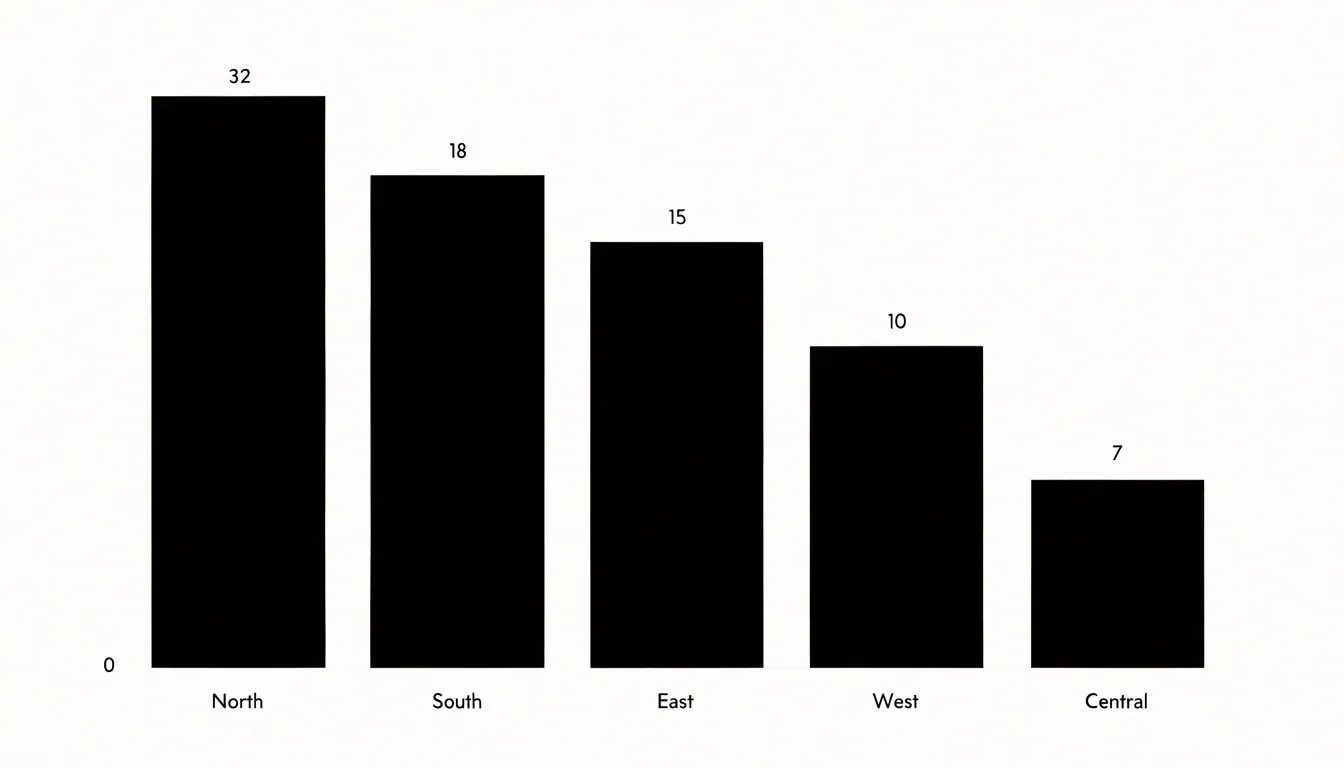
The standard vertical bar layout places categories along the horizontal axis and values along the vertical axis. Height becomes the visual encoding of magnitude, and the human eye is remarkably good at comparing heights when the bars share a common baseline. Starting every bar at zero preserves the proportional relationship between values, so a bar that is twice as tall represents twice the quantity. Readers can scan across the chart and rank categories almost instantly, which is exactly the kind of fast comparison rankings call for.
Bar charts also accommodate comparison across time periods when those periods are treated as categories. Monthly sales figures, quarterly revenue, or year-over-year counts can each occupy a bar, allowing readers to see seasonal patterns and trend direction without the assumption of continuity that a line chart imposes. Grouped or stacked variants extend the format when each category contains subcategories, though the simple single-series bar chart remains the clearest choice when the message is straightforward ranking.
Horizontal bars offer an alternative orientation that works especially well for long category labels or large numbers of categories, since the labels can run along the left edge without overlapping. Regardless of orientation, the core strength of the bar chart lies in its honesty and accessibility: the encoding is direct, the comparison is immediate, and the ranking emerges from the data itself.
Radar Charts
A radar chart, sometimes called a spider or star diagram, displays multivariate data by plotting each attribute along its own axis radiating outward from a shared center. Every axis shares the same radial scale, and the values recorded for a given item are connected with a line that encloses a filled polygon. The resulting shape acts as a visual signature for that item, making it possible to read the overall profile at a glance.
This structure suits situations where several attributes need to be evaluated together. A common use is performance profiling, for example charting an athlete across speed, endurance, strength, agility, and reaction time. Each quality occupies its own spoke, and the polygon reveals whether the profile is balanced or spiked toward particular strengths. The same logic applies to comparing features between products, assessing employee competencies, or scoring suppliers on cost, quality, delivery, and service. Because every item is plotted against identical axes and scales, the shapes can be superimposed or placed side by side, letting viewers spot which attributes drive the difference between options.
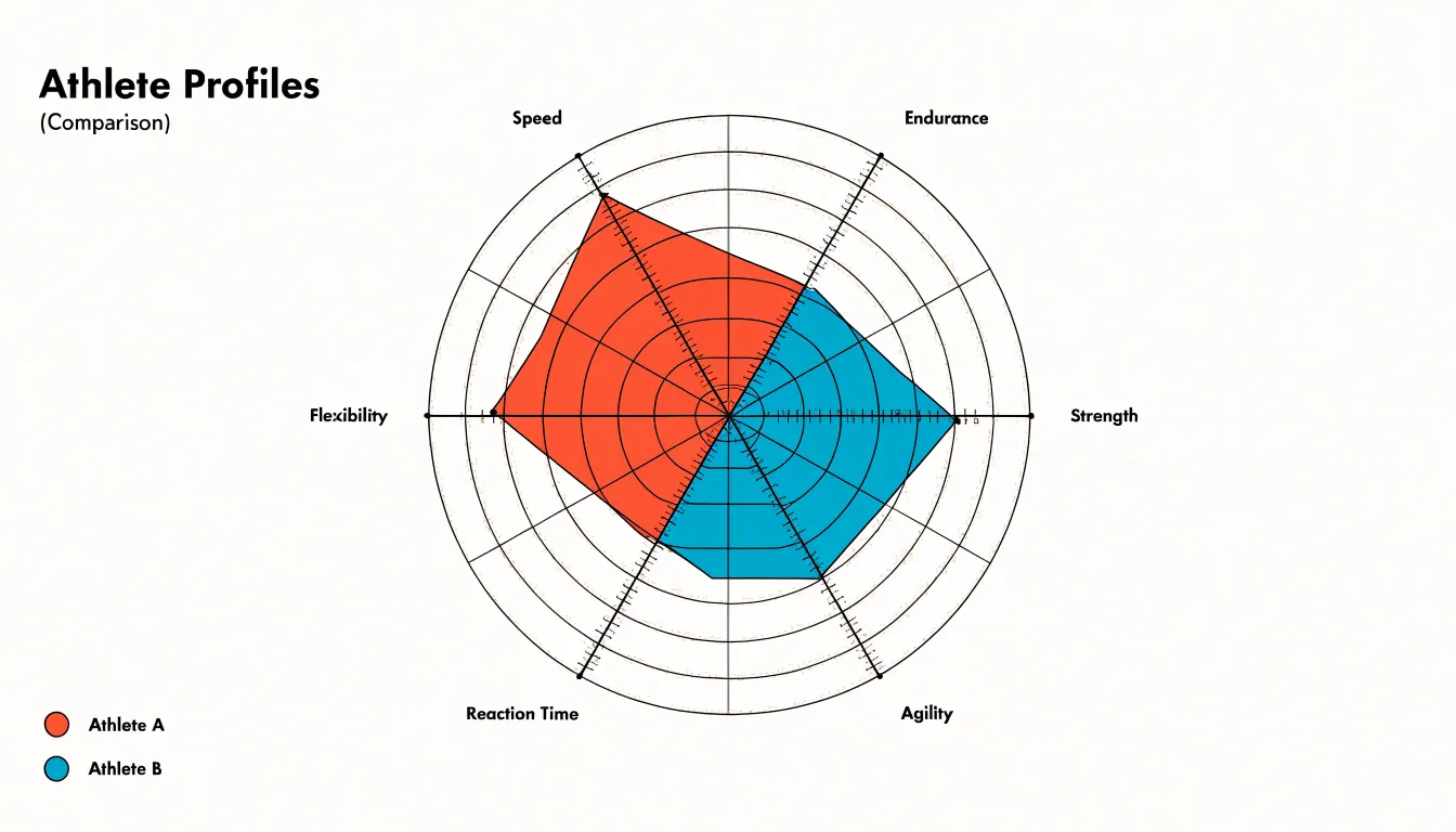
A useful detail is calibrating the radial scale carefully. When all axes share a common maximum, shapes are directly comparable; when each axis is normalized independently, charts show relative standing instead. Labeling the spokes clearly and keeping the number of axes moderate, perhaps between five and eight, preserves legibility. Consistent ordering of the axes across charts in a series further helps readers track each attribute quickly.
Radar charts work best for highlighting overall shape and balance rather than precise values. They invite the reader to compare silhouettes, note where one polygon extends beyond another, and see which attributes pull a profile outward.
Stacked Column Charts
Stacked column charts build each vertical bar from a series of segments, so the full height of the column represents a total while the individual pieces within it represent the sub-groups that make up that total. This structure makes the chart useful whenever a reader needs to understand two things at once: the overall size of each category and the internal composition that produces it. A common application is comparing departmental budgets across several years, where each column is a year and each segment is a department; the column height shows total spending, and the colored bands reveal how priorities shifted within that total. The same logic applies to sales by region broken down by product line, or survey responses by demographic group broken down by answer choice.
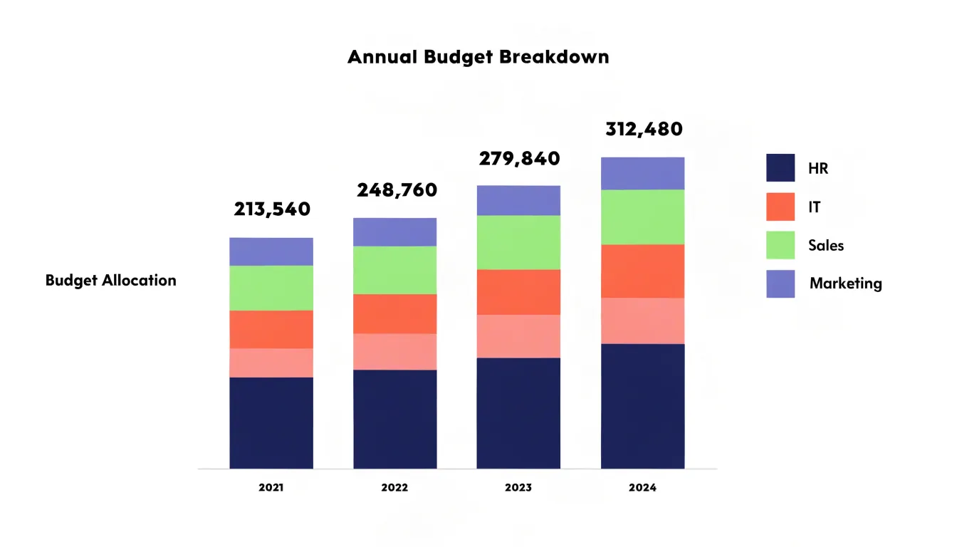
The order of the segments matters for readability. Placing the largest or most stable segment at the base of each column gives the eye a consistent anchor, while smaller segments can stack above without making the chart feel unstable. Consistent color assignments across all columns allow readers to track a single sub-group from one category to the next, and a legend positioned close to the chart reduces the effort of decoding the segments. When one sub-group dominates most columns, a 100 percent stacked variant can shift attention from absolute totals to proportional shares, though the standard stacked form remains preferable when total magnitude is itself part of the story.
Stacked columns work best with a modest number of categories and sub-groups. Too many thin slices in each column create visual clutter, and very small segments become difficult to compare with precision. Limiting the stack to four or five segments, and reserving detailed breakdowns for a companion table, keeps the chart legible.
Scatter Plots
A scatter plot places each item on a coordinate grid, with one continuous numeric measure running along the horizontal axis and another running along the vertical axis. Each mark represents a single observation, positioned according to its values on both measures. When analysts need to know whether higher values on one measure tend to accompany higher values on another, the scatter plot answers the question directly through the shape formed by the points.
The overall pattern of marks reveals correlation. Points that cluster along a rising diagonal indicate a positive relationship, while a descending band suggests a negative one. A loose, rounded cloud signals little or no association. Trends can be read from the density and direction of the cluster, and because every observation appears individually, the plot preserves the full distribution rather than compressing it into summary statistics.
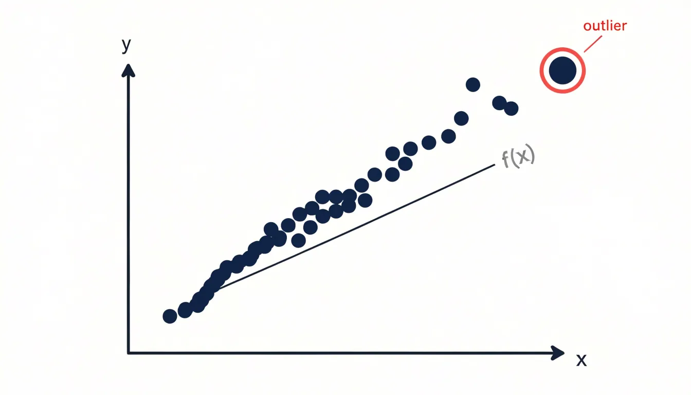
Outliers stand out naturally on a scatter plot. A point that sits far from the main cluster draws attention immediately, inviting investigation into why that item behaves differently. In ranking contexts, this is valuable for spotting organizations, products, or regions that perform unusually well or poorly on one measure relative to the other.
Scatter plots also support comparison across categories when marks are color-coded or shaped differently, allowing several groups to be examined on the same grid. With careful axis scaling and clear labeling, the chart becomes a compact tool for exploring how two measures move together, where the bulk of observations concentrate, and which individual cases deserve closer inspection before conclusions are drawn.
Line Graphs
Line graphs serve as one of the most effective tools for tracking changes over time, particularly when the underlying data is continuous and measured across regular chronological intervals. Each point on the line represents a value recorded at a specific moment, and the connecting line traces the relationship between those points, making it easy for readers to follow a sequence of events from left to right. This continuous structure allows viewers to perceive movement and direction at a glance, whether a metric is climbing steadily, holding flat, or slipping downward across weeks, months, or years.
A gradual upward slope can reveal sustained growth, while a series of peaks and troughs can expose recurring cycles tied to seasons, fiscal quarters, or promotional periods. Seasonal shifts become especially visible when the chart spans a full cycle, since the shape of the line repeats in a recognizable rhythm and draws attention to the timing of highs and lows. By plotting multiple lines on a shared axis, analysts can compare several trends side by side and observe how they converge, diverge, or move in parallel.
Growth trajectories also benefit from the line graph’s visual continuity. A sharp spike or sudden drop appears as a steep segment, while a plateau registers as a horizontal stretch, giving readers an intuitive sense of pace and momentum. When designing these charts, it helps to keep the horizontal axis evenly spaced and label time markers clearly, so the rhythm of the data stays legible. Limiting the number of lines and using distinct colors ensures each trend remains easy to follow.
Maps
Maps communicate data tied to geography by drawing on the mental model of places and distances viewers already carry into the chart. When rankings or comparisons vary by region, plotting values on a map lets audiences see clusters, gaps, and gradients at a glance rather than scanning a table of place names.
Choropleth maps assign colors or shading to defined areas such as countries, states, or counties, making them well suited to rates and normalized measures like population density, unemployment percentage, or average test scores. Because shading implies a continuous scale, choropleths work best when the regions are roughly comparable in size and the data is expressed as a proportion rather than a raw count, which prevents large areas from visually dominating simply because they cover more ground.
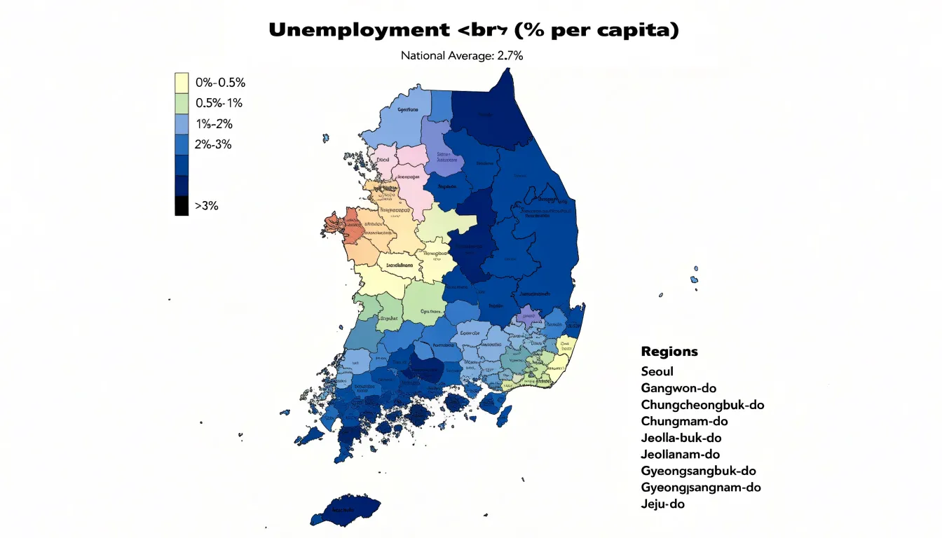
Point maps take a different approach, placing markers at specific coordinates to show the location of individual events, facilities, or customers. They excel at revealing density, dispersion, and outliers, and they handle uneven geography more gracefully than shaded regions. Many analysts combine both approaches, layering points over a choropleth to show local detail within a broader regional pattern.
Visualizing regional performance variations with maps supports comparisons across territories, highlights spatial patterns such as north-south divides or urban-rural contrasts, and helps stakeholders spot underserved areas. A thoughtful map includes a clear legend, a sensible color scheme that reads well for colorblind viewers, and a projection appropriate to the data’s scale. Labels and annotations should guide interpretation without cluttering the view.
Donut Charts
Donut charts present part-to-whole relationships through a circular ring divided into segments, with a hollow center that distinguishes them from standard pie charts. This empty middle serves a practical purpose: it can host callout metrics, key performance indicators, or short labels that summarize the chart’s message at a glance. The ring’s segments are typically sized by their percentage share, making it easy to compare relative sizes when there are only a few categories.
For instance, to display the market share of three competitors, a donut chart with three segments can instantly convey each company’s portion, while the hollow center displays the total market value or the leading company’s share. Similarly, a donut chart can highlight a single key metric, such as the percentage of users who completed a task, by filling most of the ring and leaving a small gap for the remainder, with the completion rate in the center.
Donut charts work best when the number of segments is limited, typically between two and five. Because the hollow center naturally draws attention and can hold a headline figure, donut charts are a compact, space-efficient choice for dashboards or reports where a quick proportional summary is needed.
Heat Maps
A heat map arranges data into a grid of rows and columns, where each cell corresponds to a combination of two categorical dimensions. One category runs along the horizontal axis and another along the vertical, and each intersection holds a value. Color intensity represents that value, with darker or more saturated shades typically marking higher numbers and lighter or cooler shades marking lower ones. This encoding turns an abstract matrix of figures into a visual surface that the eye can scan almost instantly.
Reading a table of numbers requires deliberate, cell-by-cell comparisons, and subtle differences between values are easy to miss. With color, clusters of similar values appear as blocks of consistent shade, and outliers stand out as contrasting spots against their neighbors. A reader can spot a hot streak along a single row, a cold column, or a diagonal band of high values before reading a single number. These patterns often point to underlying relationships between the two dimensions, such as a category that performs well only under certain conditions.
Color scales need careful handling. Sequential scales suit data that moves in one direction from low to high, while diverging scales help when values sit above and below a meaningful midpoint. Legends should make the mapping between color and value explicit so readers can translate shades back into quantities. Labeling rows and columns clearly, and ordering them thoughtfully rather than arbitrarily, further supports fast comparison.
Heat maps work well for dense matrices, such as performance across many categories, timing patterns across days and hours, or correlations between variables.
Horizontal Bar Charts
When each bar extends left to right across the page, the category name sits along the vertical axis with room to breathe, so phrases, respondent quotes, or full job titles remain readable without turning at an angle. This preserves legibility in ranked lists, survey responses, and any data set where the descriptions themselves carry meaning for the reader. Survey responses benefit most, since open-ended answers often run to several words and would crowd a vertical axis. The orientation also leaves generous space for value labels at the end of each bar, so readers can read exact figures alongside the visual comparison without hunting through the chart body.
The layout scales gracefully as the number of items grows. Rows stack vertically in order of magnitude, and a reader can follow the ranking from first to last with a steady downward gaze. Sorting the bars from largest to smallest turns the chart into a clear statement of priority, and the eye naturally settles on the top entries. When labels vary widely in length, the alignment along a common baseline keeps the chart column tidy while the bars themselves carry the quantitative signal.
Keep bar thickness consistent, leave adequate spacing between rows, and anchor the value axis at zero so the encoded lengths stay honest. Choose a muted palette or a single accent color for emphasis, letting color highlight a specific item rather than decorate the whole chart.
Pie Charts
Pie charts show how individual components combine to form a single whole. Each slice corresponds to one category, and the angle of that slice reflects that category’s proportion of the total. This makes pie charts a natural fit for questions such as how a budget splits across departments, how a customer base divides among regions, or how survey respondents distribute across a handful of answers.
The visual logic of a pie chart depends on the audience comparing angles and arc lengths, which people do with reasonable accuracy when the number of slices stays small—five or fewer distinct categories. Beyond that threshold, slices become thin, labels crowd together, and the eye struggles to distinguish similarly sized segments. When a dataset contains more categories than this, grouping the smallest ones into an ‘Other’ slice can preserve readability while still accounting for the full total.
Arranging categories from largest to smallest, usually starting at the twelve o’clock position and moving clockwise, gives viewers an immediate sense of relative magnitude and takes advantage of a reading pattern most people find intuitive. Consistent color assignments across related charts help viewers carry their understanding from one figure to the next.
Placing category names and percentage values near their slices, or in an adjacent legend, removes the guesswork of matching colors to meanings. A pie chart also depends on representing a static snapshot, since each slice describes a share at one moment in time. When the underlying proportions shift over multiple periods, a different format such as a stacked bar or line chart communicates change more clearly.
Comparison Tables
Comparison tables organize exact values into rows and columns so that readers can look up precise numbers without estimation. A table places each entity of interest in a row and each metric in a column, letting the eye travel across a single line to gather every figure attached to one item. This structure serves situations where the specific value matters more than the overall pattern, such as reporting quarterly revenue figures to two decimal places, listing the memory and processor specifications of competing hardware, or publishing the scores that determined a final ranking. Charts simplify by encoding values as lengths, angles, or positions, and that encoding inevitably involves approximation; a table removes the approximation entirely, giving the reader direct access to the underlying number.
Structured tabular data also supports multi-metric evaluation, since a wide table can hold dozens of columns covering cost, performance, reliability, and satisfaction side by side, allowing a reader to scan horizontally for one candidate or vertically for one metric. Sorting and conditional formatting extend this capability, highlighting the highest value in a column or flagging entries that exceed a threshold.
Detailed auditing represents another core use, because tables preserve the full record that produced a summary: a financial report can show line items behind a total, a survey appendix can list individual response counts, and a ranking table can include the raw inputs alongside the final position. Readers who need to verify a claim, reconcile a figure, or check how a rank was computed can follow the numbers cell by cell.
Bubble Charts
Bubble charts take the two-dimensional scatter plot and add a third dimension of information through the size of each plotted marker. The horizontal and vertical axes continue to carry two quantitative variables, while the area of each bubble represents a third measure. Readers can therefore scan a single view to see how entities compare on three metrics at the same time, for example revenue on the x-axis, growth rate on the y-axis, and market share encoded in bubble size. This makes bubble charts a natural choice when rankings depend on more than one factor and a simple ranked list would flatten important context.
Bubble size must be scaled carefully so that readers perceive differences accurately. The relationship between the underlying value and the rendered area should stay proportional, which means the radius is adjusted rather than the diameter alone. A legend showing reference circles at meaningful values gives readers an anchor for interpretation. Labels placed inside or beside the larger bubbles help identify the key entities without forcing readers to trace a separate key.
With three measures in play, visual clutter becomes the main risk. Larger bubbles can overlap smaller ones and obscure important data points, and too many entities turn the chart into a dense field of circles. Reducing the number of plotted items, applying transparency, or using outlines for overlapping markers helps preserve legibility. Colors can be reserved for categorical groupings, which introduces a fourth variable without overwhelming the chart when it is used sparingly.
In ranking contexts, the combination of position and size allows several performance dimensions to be weighed together. A company with modest x and y values but a large bubble may rank highly on scale, while a small bubble in the upper right signals efficiency.
Scorecards
Scorecards give executive stakeholders a fast, reliable snapshot of performance against the metrics that matter most to the organization. At their core, scorecards display headline numbers alongside their associated targets, making it immediately clear whether a given measure is on track, ahead, or falling behind. A well-designed scorecard pairs each metric with a percentage change or variance so readers can see both the current standing and the direction of travel without digging into underlying detail.
The value of a scorecard lies in its restraint. Executives reviewing a weekly or monthly status update need a small set of carefully chosen indicators rather than an exhaustive dashboard. Each number should answer a specific question about business health, such as whether revenue is meeting plan, whether customer satisfaction is holding steady, or whether operational efficiency is improving. Including targets alongside actuals transforms a raw number into a meaningful judgment about performance.
Percentage changes add context that absolute values alone cannot provide: a headline number shows the current level, the target shows the intended level, and the percentage change shows momentum and whether the gap is closing.
Visual hierarchy matters a great deal in scorecard design. The most important figures should dominate the layout, with supporting context presented in smaller type or secondary positions. Consistent formatting across metrics, such as aligned columns for actual, target, and variance, helps readers scan the scorecard quickly and compare entries without effort. Color can reinforce status, though it should be used sparingly and consistently so that the signal remains clear.
Dashboards
Dashboards bring several views together in a single, cohesive interface so that a ranking or comparison can be examined from multiple angles at once. Rather than isolating one chart, a well-built dashboard arranges complementary chart types side by side: a horizontal bar chart to rank items, a line chart to show how those ranks shift over time, a heat map to reveal patterns across categories, and a scatter plot to expose the relationship between rank position and a second measure. Each view answers a different question, and together they create a fuller analytical picture than any single chart could provide.
Filters, cross-highlighting, and shared axes let a viewer select an item in one chart and immediately see how it appears in the others, tracing a top-ranked product, region, or team through every dimension on display. This connected layout supports context-driven data storytelling: the presenter can move from an overview of the full ranking to a focused comparison of the top performers, then drill into the details behind a specific position, all within one environment.
The most effective dashboards follow a logical hierarchy, placing the summary ranking at the top or left and supporting detail around it, while consistent color encoding and aligned scales keep the charts readable as a set. Too many views crowd the layout; a focused selection of complementary charts keeps attention on the comparison that matters.
Frequently Asked Questions
When should I use a bar chart instead of a line graph?
Use bar charts for discrete categorical data where categories are distinct and the goal is to compare magnitudes at a glance; bar charts can also treat time periods as categories. Line graphs are for continuous data measured over regular chronological intervals.
How many axes should a radar chart have?
Keeping the number of axes moderate, perhaps between five and eight, preserves legibility. Label the spokes clearly and keep consistent ordering of the axes across charts in a series.
What are stacked column charts best used for?
Stacked column charts show both the overall size of each category and the internal composition that produces it, such as departmental budgets across several years. Limiting the stack to four or five segments helps keep the chart legible.
How can you tell if there is a correlation on a scatter plot?
Points that cluster along a rising diagonal indicate a positive relationship, a descending band suggests a negative one, and a loose, rounded cloud signals little or no association. Outliers sit far from the main cluster and draw attention immediately.
What is the difference between a choropleth map and a point map?
Choropleth maps assign colors or shading to defined areas and work best for rates and normalized measures, while point maps place markers at specific coordinates to show individual events, facilities, or customers. Point maps reveal density, dispersion, and outliers.
What should a performance scorecard include?
Scorecards display headline numbers alongside their associated targets and pair each metric with a percentage change or variance. They should use a small set of carefully chosen indicators rather than an exhaustive dashboard.
Tony Astor
Tony writes about data visualization and the tools people use to build charts and dashboards. More about Data Illustrator