How to Visualize Percentages and Rates
 By Tony Astor ·

How to Visualize Percentages and Rates
Waffle charts show a percentage by filling a 10×10 grid of 100 squares, with each square representing one percent. A value of 37 percent fills 37 squares; the rest stay neutral. Because the grid always totals 100, proportions are read directly without axes, scales, or legends, making them intuitive for single percentages and progress metrics.
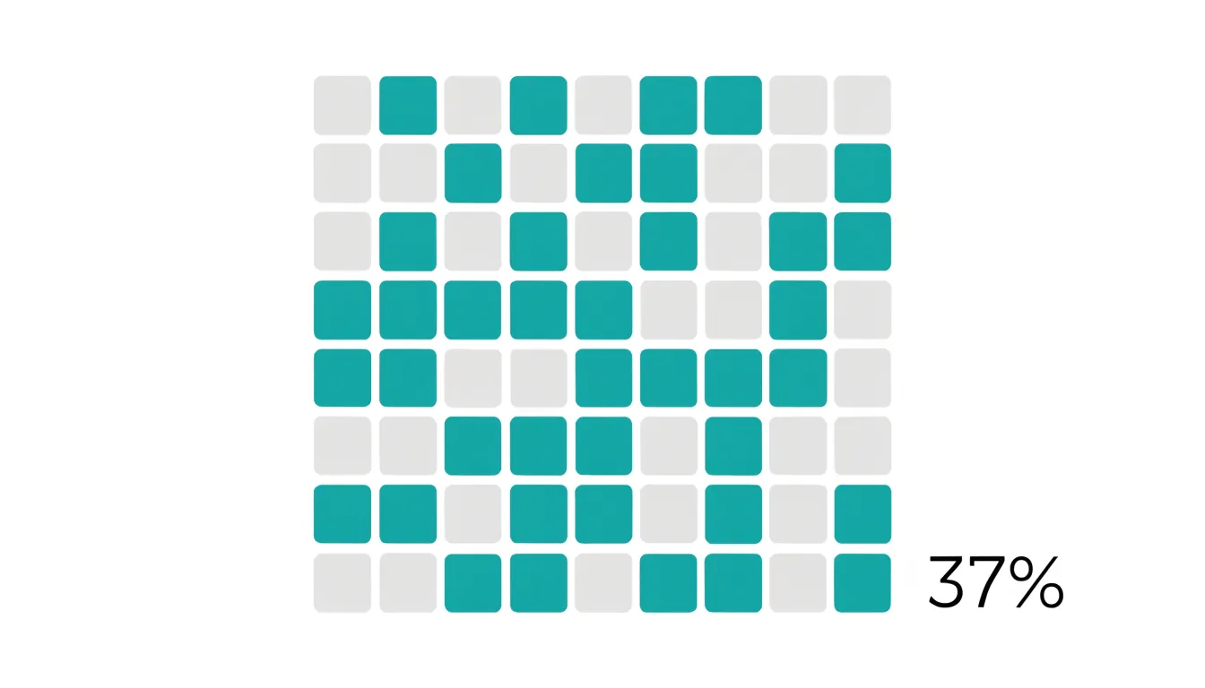
Table of Contents
Pie Charts
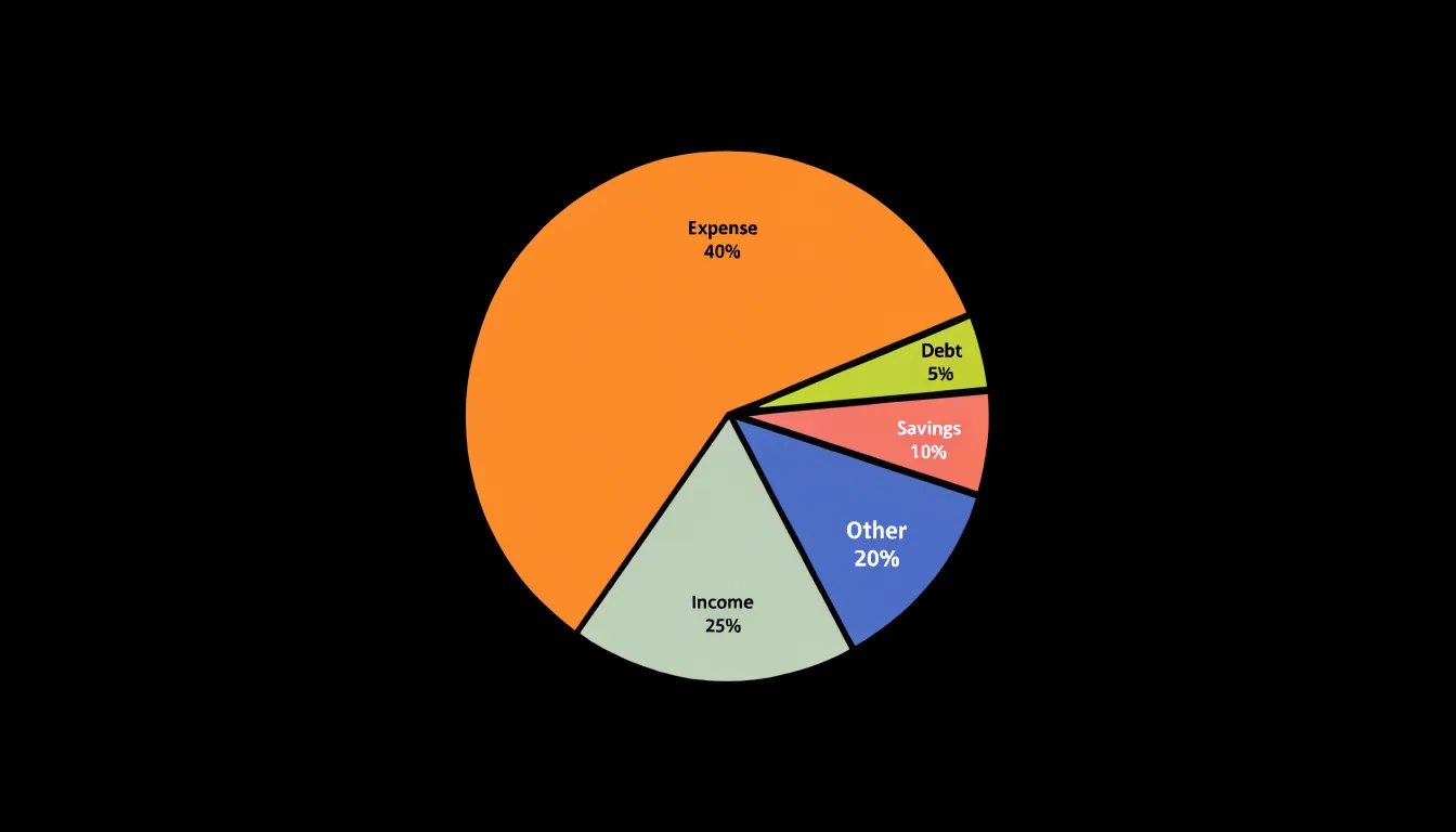
Pie charts excel at showing simple part-to-whole relationships when the number of categories is small. With five or fewer slices, viewers can quickly grasp the relative size of each component without mental effort. The circular shape naturally suggests a whole, and each slice’s angle directly corresponds to its percentage, making proportions intuitive. To maximize clarity, start the first slice at the 12 o’clock position and arrange the remaining slices clockwise in descending order of size. This convention aligns with how most people read a clock and ensures the largest segments are most prominent. Label each slice directly with its category name and percentage, either inside the slice if it is large enough or just outside with a leader line. Use a limited color palette with distinct hues that are easy to differentiate, and avoid patterns or gradients that can obscure the data. Keep the design clean by removing unnecessary borders, shadows, and 3D effects, which distort perception. When two or more slices are very similar in size, consider adding a callout or a secondary chart to highlight the difference, as pie charts are less effective at showing fine distinctions. Also, ensure that the total adds up to 100% and that the slices are clearly separated by thin white borders for readability. By following these best practices, a pie chart becomes a powerful tool for quickly communicating proportional distributions in reports, presentations, and dashboards, especially when the audience needs a fast, at-a-glance understanding of how individual parts contribute to the whole.
Waffle Charts
A waffle chart represents a percentage by filling a ten-by-ten grid of one hundred small squares, with each square standing for one percent of the total. To show a value of 37 percent, thirty-seven squares are filled in a contrasting color while the remaining sixty-three stay in a light neutral tone. Because the grid always contains exactly one hundred cells, the reader can see the proportion directly without needing to interpret an axis, a scale, or a legend. This makes the format especially approachable for audiences who may find abstract charts difficult to parse at a glance.
The structure of the waffle chart carries several practical benefits. Counting squares comes naturally to most viewers, so a filled block of cells reads almost like a row of tally marks that has been neatly arranged into a square. The ten-by-ten layout also makes it easy to estimate fractions of the whole, since each row or column represents ten percent. Readers can quickly see that a half-filled grid means fifty percent, or that three complete rows equal thirty percent, which supports fast mental arithmetic and comparison.
Waffle charts work particularly well for single percentages and completion metrics. A progress report showing how many tasks have been finished, a dashboard tracking a fundraising target, or a summary of survey responses can all use the grid to communicate a figure with immediate clarity. The visual weight of the colored area provides an honest impression of magnitude, so a small percentage looks small and a large one looks dominant. This intuitive sense of scale helps prevent misreading, particularly compared with charts that stretch or compress their axes.
Accessibility is another strength of the format. The regular grid of identical shapes is simple to describe in words or in alt text, and the clear contrast between filled and empty cells aids readers with low vision. When space allows, adding the numeric value alongside the grid reinforces the message for everyone.
Bar Charts
Bar charts earn their reputation as the gold standard for comparing categorical rates because they align directly with how people read and judge magnitude. Each bar begins from a common baseline, typically zero, and extends outward in proportion to the rate it represents. That shared starting point means the visual length of a bar maps onto the underlying number, so a rate that is twice as large produces a bar that is twice as long. Readers can rank categories at a glance, spot the largest and smallest values immediately, and estimate ratios between bars without consulting the axis labels. Horizontal bars orient the categories along the vertical axis, giving long category names room to breathe, while vertical bars suit shorter labels and fit naturally into dashboards and report pages. Both formats perform the same core job, and the choice between them usually comes down to label length and layout constraints.
The format also shines when the timeframe is held constant. When every category is measured over the same period, the only variable left to compare is the rate itself, and bars isolate that comparison cleanly. The eye moves from bar to bar, measuring differences in length rather than area or angle, which are harder to judge accurately. Sorted bars, ordered from highest to lowest, turn a chart into an instant ranking and make outlier categories stand out. Small multiples of bar charts extend the approach across several timeframes or segments while preserving the same visual grammar, so patterns remain comparable across panels. For audiences who need precise, honest comparisons of distinct categorical rates, bars offer a balance of clarity, accuracy, and accessibility that few alternatives match.
Stacked Bar Charts
Stacked bar charts are a natural fit for part-to-whole relationships because each bar represents a complete whole, usually 100 percent, while the segments within it show how that whole divides among sub-components. To build one, start with a categorical axis holding the comparative groups, such as regions, time periods, or product lines. Each group receives a single bar scaled to the full total, and the bar is divided into colored segments whose lengths correspond to the share each sub-component contributes. Because every bar spans the same total, readers can compare internal composition across groups at a glance: a segment that swells in one bar and shrinks in another immediately signals a shift in proportion. Ordering segments consistently across all bars, ideally from largest to smallest or in a fixed logical sequence, keeps the eye from re-learning the layout for each group. Labeling segments directly with their percentages, rather than relying solely on a legend, reduces the back-and-forth between chart and key, and placing the largest or most important segment at the base of each bar anchors the comparison. When many sub-components exist, group the smallest into a single residual category to prevent slivers that are too thin to read. A 100 percent stacked bar works best when the underlying totals vary widely and the question concerns relative share rather than absolute size; for cases where both the total and the composition matter, annotate each bar with its raw total. Consistent color meaning across groups, accessible contrast between adjacent segments, and a clear horizontal baseline complete the design, allowing viewers to trace how each sub-component’s contribution changes from one group to the next.
Donut Charts
The donut chart takes the familiar ring of a pie chart and opens up its center, creating a dedicated space for information that would otherwise compete with the slices themselves. That cutout serves a practical purpose: it gives you a natural anchor for a headline number. When you place a single summary figure inside the ring, such as a total count, an overall rate, or an average, the chart communicates both the parts and the whole in one compact graphic. The reader’s eye moves first to the central value, then outward to the slices, which means the most important statistic frames everything else on the page.
The proportional segments around the ring retain the same intuitive reading that pie charts offer. Each slice’s angular span corresponds directly to its share of the total, so audiences can estimate relative sizes without consulting a legend or table. The proportions stay legible because the ring keeps a constant width, and the uniform distance from the center makes differences between adjacent slices easy to compare. Many designers also add direct percentage labels along the ring, which further reduces guesswork and keeps the chart readable at smaller sizes.
The visual restraint of the donut format helps when several charts appear together on a dashboard or report page. The hollow center creates breathing room, so a series of small donut charts feels less crowded than an equivalent row of pies. Colors can be limited to a few meaningful hues, with the remaining categories grouped into a neutral tone, and the central figure can carry the color accent that ties the whole graphic together. These choices keep attention on the summary value while the ring does the quieter work of showing composition. Used this way, the donut chart balances a clean, modern appearance with faithful representation of percentage data.
Line Graphs
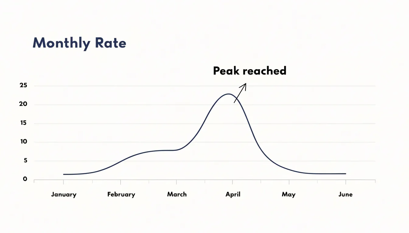
Line graphs excel at revealing how rates evolve across a continuous time axis. By plotting a metric at regular intervals—daily, monthly, or quarterly—the line connects individual data points into a trajectory that shows fluctuations, turning points, and long-term direction. This continuous representation makes it straightforward to spot seasonal patterns, such as recurring spikes in retail sales each December or dips in website traffic during summer holidays. The slope of the line at any segment conveys growth velocity: a steep ascent indicates rapid acceleration, while a flattening curve suggests deceleration or stabilization. Viewers can quickly compare the pace of change between periods, identifying when a rate is speeding up or slowing down. Unlike bar charts, which emphasize discrete comparisons, line graphs highlight the flow of change, making them ideal for time-series data where the order and spacing of observations matter. When multiple series are plotted on the same axes, relative performance becomes visible—for instance, comparing the conversion rates of two marketing campaigns over several months. However, effective line graphs require careful design: consistent intervals on the time axis, clearly labeled units, and a scale that neither exaggerates nor obscures variation. Overcrowding with too many lines can clutter the view, so limiting to a few key series or using small multiples often works better. By focusing on the shape of the line, viewers can discern trends that might be hidden in tables of numbers, making line graphs a powerful tool for communicating how rates change over time.
Area Charts
Area charts build on the familiar line chart by shading the region between the trendline and the baseline, turning a simple trajectory into a statement about accumulated magnitude. Where a bare line communicates direction and pace, the filled space beneath it communicates volume: every point along the horizontal axis carries with it the total quantity that has built up to that moment, and the visible mass of color makes that accumulation legible at a glance. This quality makes area charts particularly effective when the story you want to tell concerns sustained growth, persistent decline, or the slow compounding of small daily or monthly increments into something substantial over a quarter or a year.
The filled region also supports comparison of relative proportions across time. When several areas are stacked, the height of each band at any given point shows its share of the whole, and the overall silhouette shows how the combined total swells or contracts. A viewer can trace a single category’s band as it widens through one season and thins through another, reading both its absolute contribution and its changing prominence without consulting a table. This layered reading suits topics such as revenue by product line, energy consumption by source, or traffic segmented by channel.
Design choices matter a great deal with area charts. Transparency in overlapping fills keeps smaller layers visible, and a sensible ordering of stacked series—usually largest at the bottom—prevents the eye from being misled about proportions. Gridlines should be light so the filled shapes dominate. Used with care, area charts reward sustained attention: they let an audience feel the weight of cumulative trends rather than merely noting their direction.
Progress Bars and Gauges
Progress bars and gauges translate a single value into a visual position along a defined scale, which makes them well suited to showing how far a metric has moved toward a fixed target. A linear progress bar maps a percentage onto a horizontal or vertical track, so a viewer can read completion at a glance without parsing numbers. A radial gauge performs the same mapping around an arc, often with a needle or filled segment indicating the current reading against labeled tick marks. Both forms share a core strength: they anchor a value to a known endpoint, so the distance remaining is as visible as the distance covered.
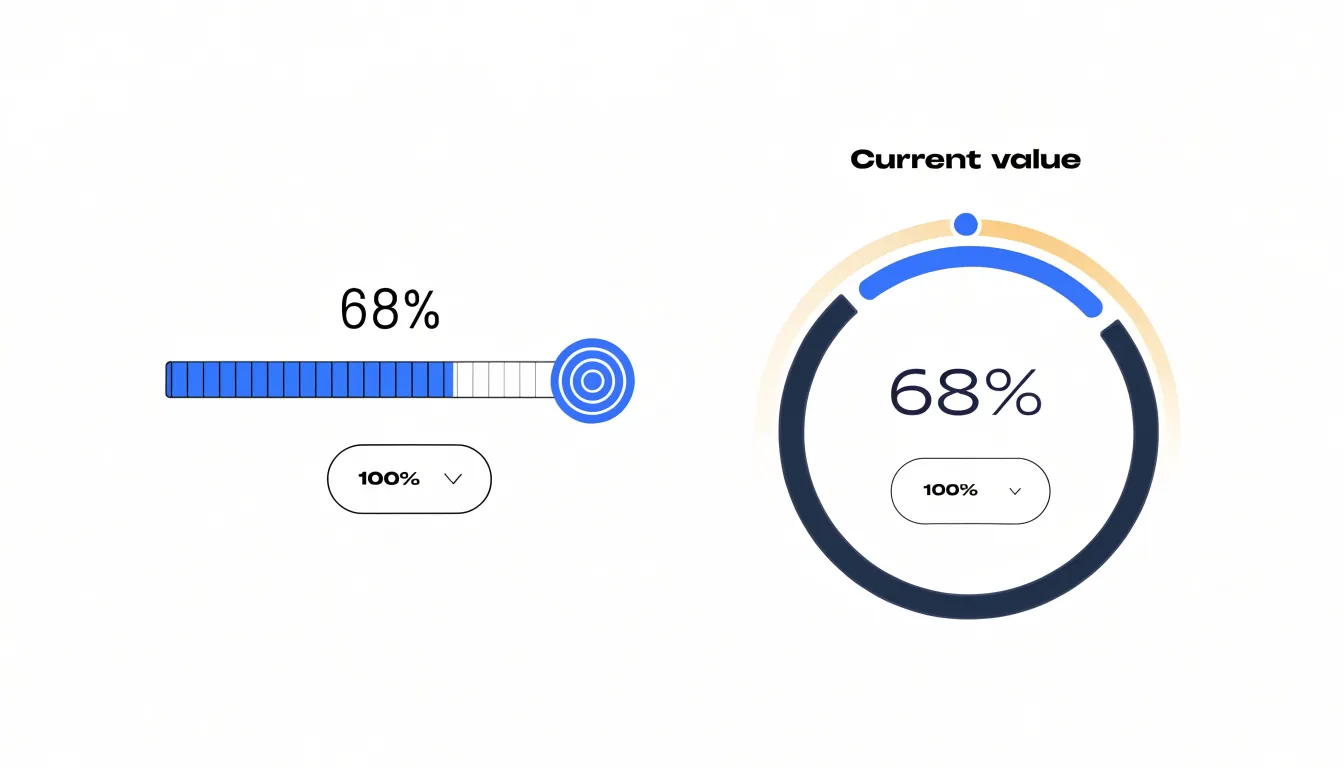
These indicators work best when the target is stable and the metric is singular. A fundraising campaign tracking dollars against a goal, a download counter approaching a fixed file size, or a service dashboard showing uptime against an agreed threshold all benefit from this treatment. Real-time status updates suit progress bars and gauges particularly well, since the fill level or needle position can shift continuously as new data arrives, giving viewers an immediate sense of momentum or shortfall. Color can reinforce the message, with a change in hue signaling that a threshold has been crossed.
Design choices matter for accuracy. A linear bar with clear start and end points reads precisely because its length is proportional to the value. Gauges carry more visual weight but can obscure fine differences near the ends of the arc, so they suit contexts where approximate position is enough. Labeling the current value and the target directly on the graphic removes ambiguity, and consistent scaling across a set of indicators lets viewers compare them fairly. Used with care, progress bars and gauges turn abstract percentages into spatial relationships that audiences grasp quickly and remember.
Treemaps
Treemaps offer a compact way to display hierarchical data in which each part-to-whole relationship can be read at a glance. The chart works by dividing a rectangle into nested rectangular tiles, where every tile represents a node in a tree structure. The area of each tile is proportional to a percentage or value, so a category that accounts for 40 percent of the total occupies roughly 40 percent of the parent rectangle. Subcategories are nested inside their parent tiles, creating a visual map of the hierarchy in which the relative weight of each branch is immediately apparent.
The strength of a treemap lies in its ability to show two variables at once. Size expresses the percentage or rate that defines how much of the whole a tile represents, while color can encode a second critical measure, such as a conversion rate, growth percentage, or performance against target. A viewer can therefore scan the chart and identify large tiles that carry problematic rates, or small tiles that punch above their weight. This dual encoding makes treemaps especially useful for datasets that combine volume and efficiency, such as product categories by revenue share and margin, or regions by population share and rate of change.
Treemaps also handle multi-level structures well. A single rectangle can contain departments, which contain teams, which contain individual projects, all nested in a consistent visual grammar. This nesting preserves the context of each percentage, since every tile sits inside the boundary of its parent and its share can be read relative to that parent or to the whole. When working with complex hierarchical datasets where many categories compete for limited space, treemaps keep the display dense yet organized, allowing readers to compare rates across levels without losing sight of the overall composition. The result is a visualization that communicates both structure and performance in a single view.
Dot Plots
Dot plots encode values as points positioned along a shared axis, a design that leverages the precision of positional encoding to reveal small differences in rates. When many categories or groups are compared, a dot plot places each value as a distinct marker, allowing the eye to detect subtle shifts that might be lost in other chart types. The shared axis provides a common scale, so even minor variations in position are immediately apparent. This is particularly useful for spotting small differences in precise rates, such as percentages that differ by only a few tenths of a percent. In contrast, bar charts encode values with both position and length, and the filled area can introduce visual noise that obscures fine distinctions. The solid bars may draw attention to overall magnitude rather than exact position, and the thickness of the bar can make it harder to judge small increments. Dot plots avoid this by reducing each value to a single point, minimizing visual clutter and emphasizing the exact location along the axis. The result is a clean, uncluttered display where small statistical variations stand out. For example, when comparing rates across many categories, a dot plot can highlight which categories are slightly above or below a reference line, or which pairs differ by a small margin. This makes dot plots especially valuable for exploratory analysis, where the goal is to identify patterns and anomalies that might be missed with more conventional charts. By focusing on precise positional encoding, dot plots offer a powerful way to visualize percentages and rates with clarity and accuracy.
Heat Maps
Heat maps transform rates into visual patterns by assigning color intensity to geographic regions or matrix cells. When mapping rates across regions, each area—whether a country, state, or county—is shaded according to its value, with darker or more saturated colors typically indicating higher rates and lighter colors indicating lower rates. This creates an immediate visual impression of spatial density and concentration. For example, a heat map of vaccination rates by county can quickly reveal clusters of low coverage, while a heat map of disease incidence might highlight hotspots. The human eye is naturally drawn to areas of strong color, making it easy to spot regional anomalies such as outliers where the rate is unusually high or low compared to neighbors. Beyond geographic maps, heat maps can also be applied to matrices, such as a table of rates by age group and region, where color intensity helps identify patterns across two dimensions. The key advantage of heat maps is their ability to compress large amounts of data into a single visual that supports rapid comparison and pattern recognition. However, effective use requires careful choice of color scales—sequential palettes for ordered rates, diverging palettes when deviations from a baseline are of interest—and consideration of perceptual uniformity to avoid misleading interpretations. Additionally, rates should be based on sufficient denominators to avoid random fluctuations that can create false hotspots. When designed thoughtfully, heat maps serve as powerful tools for communicating spatial disparities and guiding further investigation into the underlying causes of regional differences.
Population Pyramids
A population pyramid organizes demographic data into a shape that readers can interpret at a glance, with age brackets stacked vertically and two sets of horizontal bars extending left and right from a central axis. The vertical dimension typically represents age groups in ascending order, from the youngest cohort at the base to the oldest at the apex, while the horizontal dimension shows the percentage of the total population falling into each age and gender combination. Because the bars are measured against the same scale on both sides, the viewer can compare male and female distributions directly and see how the proportions shift across the life course.
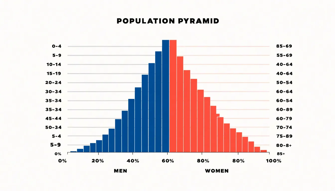
Building this visualization requires several deliberate choices. Age brackets should be uniform in width, usually five-year intervals, so that bar heights correspond to equal spans of time and the silhouette remains comparable across groups. The percentage scale on both axes needs identical increments and a shared maximum value, otherwise differences between the two sides will appear larger or smaller than they are. Labels placed at the category ticks rather than beside individual bars keep the chart readable, particularly when many age groups are present. The mirroring convention is flexible, but the chart must state clearly which side represents which gender.
The resulting silhouette carries meaning in its outline. A broad base tapering toward a narrow top indicates a young population with high birth rates and shorter average lifespans, while a roughly rectangular profile suggests stable birth and death rates with a large middle-aged cohort. Narrowing at the base alongside a wide midsection points to an aging population. When several pyramids are placed side by side for different regions or years, audiences can trace how cohorts move upward over time and where the percentage of dependents concentrates relative to the working-age population. This makes the format useful for policy planning, market analysis, and public health reporting, where the relative size of age groups often matters more than raw counts.
Dashboard
A dashboard that combines multiple rate visualizations transforms isolated metrics into a coherent narrative for strategic decision-making. The first strategy is to anchor the layout with a primary visualization that captures the most critical rate, such as overall conversion or growth, placed prominently at the top or center. Surround it with supporting visuals that provide context, like segmented rates by channel, trend lines over time, or comparative benchmarks. Group related metrics into logical zones—for example, acquisition rates on one side and retention rates on the other—to guide the viewer’s eye through the story. Use consistent color scales and labeling across all charts so that rates can be compared without confusion. Interactive elements such as filters or drill-downs allow users to explore specific segments while maintaining the overall narrative. A cohesive data story emerges when each visualization answers a question raised by the previous one, leading the viewer from summary to detail. For instance, a high-level rate might prompt a question about which segment drives it, which the next chart addresses. Strategic decision-makers benefit from clear hierarchies and visual cues that highlight anomalies or significant changes. Incorporate annotations or callouts to draw attention to key insights, and ensure that the dashboard updates dynamically with fresh data. By synthesizing diverse visual components into an interactive layout, the dashboard becomes more than a collection of charts—it becomes a tool for storytelling that guides executives toward informed actions.
Frequently Asked Questions
When should I use a pie chart instead of a bar chart?
Pie charts excel at showing simple part-to-whole relationships when the number of categories is small, ideally five or fewer slices. Bar charts are the gold standard for comparing categorical rates because each bar begins from a common baseline and extends in proportion to the rate it represents.
How does a waffle chart show a value like 37 percent?
A waffle chart uses a ten-by-ten grid of one hundred small squares, with each square standing for one percent of the total. To show 37 percent, thirty-seven squares are filled in a contrasting color while the remaining sixty-three stay in a light neutral tone.
How should I label segments in a 100 percent stacked bar chart?
Label segments directly with their percentages rather than relying solely on a legend, which reduces back-and-forth between the chart and key. Ordering segments consistently across all bars and placing the largest or most important segment at the base also helps anchor the comparison.
What chart type is best for showing how rates change over time?
Line graphs excel at revealing how rates evolve across a continuous time axis by plotting a metric at regular intervals and connecting individual data points into a trajectory. They make fluctuations, turning points, seasonal patterns, and long-term direction easier to spot.
What should I be careful about when using a heat map?
Heat maps require careful choice of color scales, such as sequential palettes for ordered rates or diverging palettes when deviations from a baseline matter. Rates should also be based on sufficient denominators to avoid random fluctuations that can create false hotspots.
What is a design limitation of gauges?
Gauges carry more visual weight but can obscure fine differences near the ends of the arc, so they suit contexts where approximate position is enough. Labeling the current value and the target directly on the graphic helps remove ambiguity.
Tony Astor
Tony writes about data visualization and the tools people use to build charts and dashboards. More about Data Illustrator