How to Visualize Likert Scale Data
 By Tony Astor ·

How to Visualize Likert Scale Data
Use diverging bar charts to visualize Likert data, splitting agreement and disagreement around a central neutral axis so each survey item’s sentiment balance is visible at a glance. Stack intensity categories within each bar, apply consistent diverging colors, sort items by net agreement, and report means alongside medians to preserve the scale’s nuance.
Table of Contents
Diverging Bar Chart
A diverging bar chart arranges each survey item as a horizontal bar split around a central axis, with one direction reserved for agreement responses and the other for disagreement. The neutral midpoint sits on the axis itself, so the eye immediately registers which side of the balance each question falls on and by how much. Respondents who agree, strongly agree, and lean positive extend to the right, while disagree, strongly disagree, and lean negative extend to the left. Because every question shares this same center line, the reader can scan down the list and compare the shape and weight of sentiment across many items without reorienting at each row.
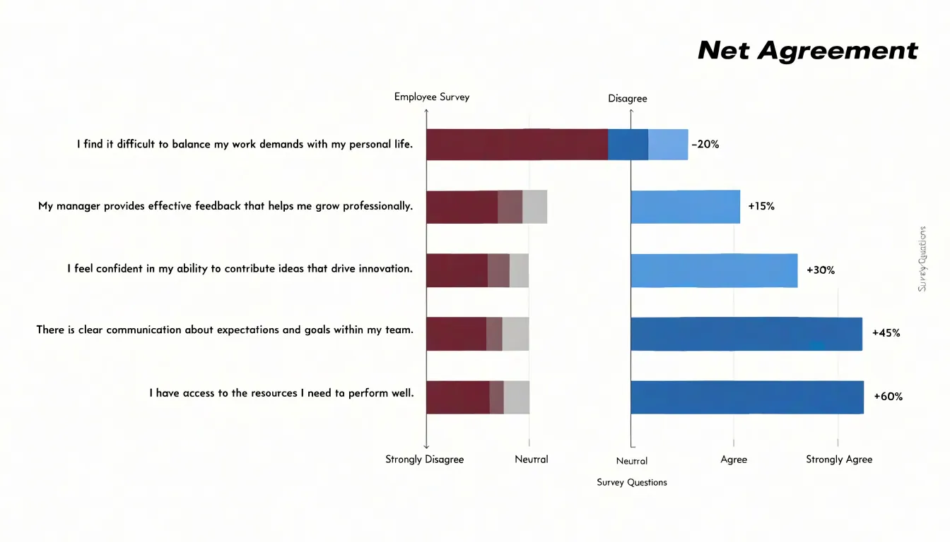
This alignment turns a table of percentages into a picture of overall mood: questions where the right side dominates read as broad endorsement, questions where the left side stretches further read as friction or concern, and questions with two roughly equal wings signal a divided audience. Stacking the intensity categories within each bar, from strong agreement at the outer tip to mild agreement nearest the axis, preserves the nuance of a Likert scale rather than collapsing it into a single number. The central axis also gives neutral or undecided responses a natural home, either as a gap at the axis or as a small centered band, so the middle of the scale stays visible instead of disappearing into rounding. Color choices reinforce the comparison when one hue marks the agreement side and a contrasting hue marks disagreement. The result is a compact, ordered view that lets a reader rank questions by sentiment balance and spot outliers in seconds, making the diverging bar chart one of the most dependable formats for summarizing multi-item survey results.
Stacked Bar Chart
A stacked bar chart presents each survey question as a single horizontal bar divided into segments, where every segment corresponds to one rating option on the Likert scale. Each bar is normalized to a total height or width of 100 percent, so the segments sit end to end and together account for all responses to that question. This structure gives stakeholders a direct visual read of the exact breakdown of every rating option, showing how much of the sample chose each point on the scale without requiring them to consult a separate table.
To build an effective 100 percent stacked chart, begin by converting raw counts into percentages within each question, then order the segments consistently across all bars. A common approach places the most negative option at one end and the most positive at the other, so readers can scan the chart and compare distributions at a glance. Assigning distinct colors to each rating point and repeating the same color mapping across every question keeps the display coherent. Labeling the segments with their percentage values, either directly inside wider segments or as small annotations near narrower ones, helps stakeholders see exact figures rather than estimating from color blocks.
Sorting the questions by the share of favorable responses surfaces which items performed best and which performed worst. Adding a thin outline around each segment, or a subtle divider between the positive and negative halves of the scale, makes the neutral midpoint easy to locate. Where sample sizes differ between questions, note the base number in a label or footnote so readers understand the context behind each bar.
Color Choices
The human eye processes hue and saturation faster than it reads labels or numbers, so color choices should mirror the natural order of the response spectrum. Two palette families serve this purpose well:
- Sequential palettes move from light to dark within a single hue, such as pale blue through deep navy. Mapping the lightest shade to strong disagreement and the darkest to strong agreement creates a visual ramp that reads as intensity, with neutral midpoints sitting naturally in the middle.
- Divergent palettes place two contrasting hues at the poles with a pale or neutral tone at the center, which suits scales that pivot around a neutral midpoint. A warm-to-cool scheme, such as orange through grey to blue, lets strong disagreement and strong agreement occupy clearly distinguishable ends while the neutral category recedes visually.
Accessibility deserves equal attention during palette selection. Around one in twelve men has some form of color vision deficiency, and red-green combinations in particular can collapse into indistinguishable tones. Divergent palettes built on blue and orange, or on purple and yellow-green, remain legible for most viewers with deuteranopia or protanopia. Avoiding reliance on hue alone strengthens the design further: varying lightness across categories means the palette still communicates order in greyscale printing or on low-quality screens. Tools such as ColorBrewer and dedicated contrast checkers make it straightforward to test candidate palettes before committing to them.
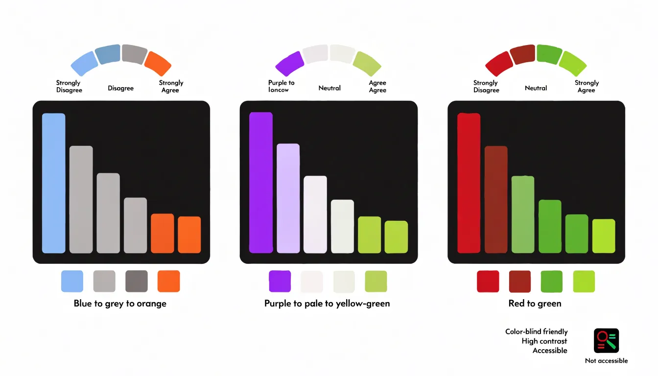
Consistency across every chart in a report matters as much as the palette itself. Once strong disagreement is assigned a color, that color should mean the same thing on every figure, so readers build a mental legend and apply it automatically.
Neutral Responses
When respondents select a midpoint option such as “neither agree nor disagree” or “undecided,” that feedback represents an absence of directional opinion. How you position these neutral responses shapes how viewers interpret the overall distribution.
Placing neutral data directly on the center baseline of a diverging chart keeps the scale structurally intact, allowing positive and negative responses to extend outward symmetrically from a shared origin. This approach preserves the natural geometry of the five- or seven-point scale, so viewers can trace each response category back to its source without confusion. The center baseline becomes both a visual anchor and a meaningful category, and the stacked or split segments remain proportional to the raw counts.
Isolating neutral responses into a separate band, gap, or dedicated column offers another path. This strategy prevents the midpoint from crowding the visual center of the chart when neutral counts are large. Pulling neutral feedback away from the divergence point lets the viewer see the strength of opinion on each side more directly, and the center no longer carries the visual weight of an ambiguous category. A separate neutral segment also makes the size of the undecided group plain at a glance, which matters when a high neutral share signals respondent uncertainty.
The choice between these strategies hinges on the analytical message. To show the full shape of the scale and maintain faithful proportional relationships, keep neutral data on the center baseline. To emphasize the balance of positive versus negative sentiment, isolate the neutral group. Either way, apply the placement consistently across all items in a chart set to prevent viewers from misreading the midpoint as a swing toward one side, and document the choice in a legend or annotation.
Average Scores
When a survey uses a balanced set of response options, such as strongly disagree through strongly agree, each option can be assigned a value from one to five. Calculating a mean across respondents yields a single figure describing the overall tendency of the group, which is useful for comparing groups, tracking change over time, or ranking items by relative agreement. For example, a mean of 3.8 on a satisfaction item signals that responses cluster toward the positive end of the scale.
Numerical averages work best when responses are reasonably spread out and roughly symmetric. Under those conditions, the mean reflects the typical respondent fairly well and allows straightforward comparison between different questions or demographic segments sharing the same numeric scale.
The picture changes when responses cluster heavily at one end of the scale or include a small number of extreme answers. A handful of strongly negative ratings can pull a mean downward, making the group appear more dissatisfied than most respondents actually are. In these situations, the median becomes the more reliable measure. Because it identifies the middle response rather than balancing all values, the median resists distortion from outliers and skewed distributions. A median of four tells you that at least half of respondents chose four or five, regardless of how extreme the remaining answers might be.
As a practical guideline, report the mean alongside the median so readers see both the central tendency and the influence of outliers. Also report the distribution of responses through frequencies or percentages to give a fuller picture of how people actually answered.
Group Comparison
Group comparison splits respondents into meaningful segments—such as demographic categories like age, region, or role, or behavioral cohorts like new versus returning users—and visualizes each segment’s response distribution side by side. This surfaces contrasts that an overall average conceals: a product may score moderately positive overall while one age bracket is enthusiastic and another is quietly dissatisfied.
Several chart formats support segmented comparisons:
- Stacked bar charts organized by segment show the proportion choosing each point on the scale, making it easy to spot where one group leans toward agreement while another clusters around neutral.
- Diverging bar charts let readers see the balance of opinion tilt left or right for each segment.
- Dot plots or small multiples display each group’s median and spread on compact dashboards without overwhelming the viewer.
Effective group comparison requires segments large enough to be statistically meaningful, consistent color encoding across all groups, and clear labeling so readers can trace which segment is which. Ordering groups by a meaningful variable, such as response rate or sample size, further sharpens the comparison and guides stakeholders toward targeted decisions.
Heat Map
A heat map transforms a standard data table into a color-coded grid, where each cell’s shade reflects the value of a specific response category. For Likert scale data, you can display every question alongside every response option (such as Strongly Disagree through Strongly Agree) and assign a color gradient to represent the percentage of respondents who selected each option.
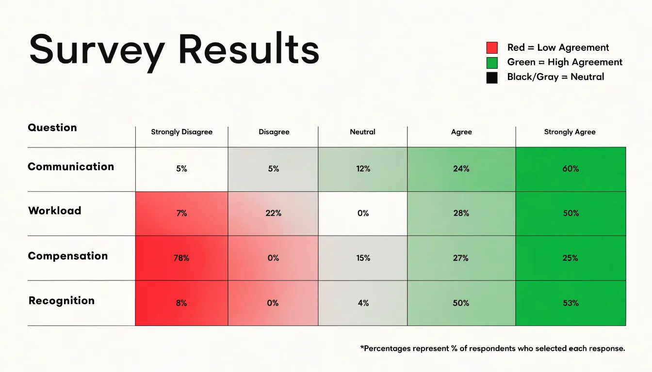
The resulting visual matrix allows you to scan dozens of questions at once and identify patterns. Dark clusters might indicate questions where most respondents chose “Agree,” while light areas could signal neutrality or low engagement. By using color density, heat maps make it easy to spot high-performing areas and problematic areas across large surveys where traditional tables become overwhelming. For instance, you might notice that questions about “communication” are predominantly green (positive), while those about “workload” are red (negative). Heat maps can also be enhanced with sorting or grouping to highlight specific sections, and they work well with diverging color scales to emphasize the polarity of responses.
Radar Chart
A radar chart, often called a spider chart, compares satisfaction profiles across multiple categories. Imagine you have surveyed employees from different functional areas—such as Sales, Marketing, Engineering, and Customer Support—and asked them to rate their overall satisfaction on a 5-point Likert scale. A radar chart plots each category along its own axis radiating from a central point, with the satisfaction scores connected to form a polygon representing each group’s profile. Overlaying multiple polygons shows which areas are performing well and which lag behind.
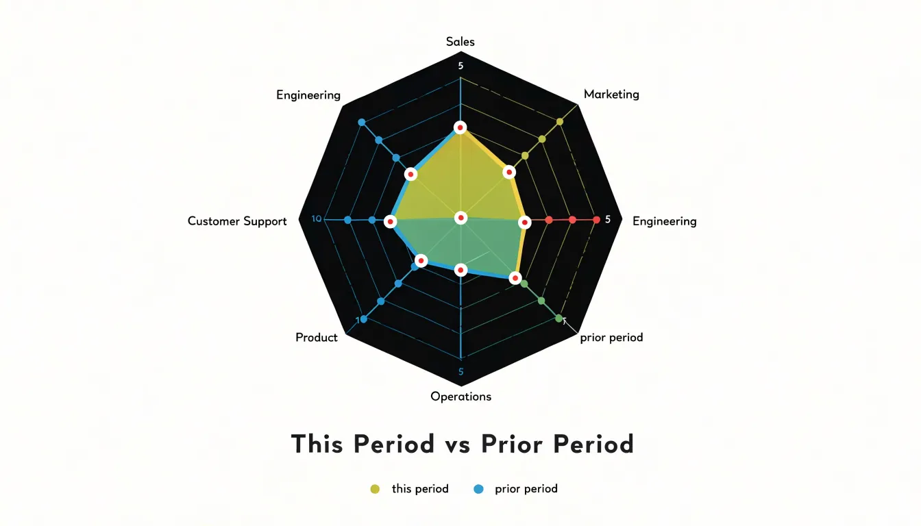
Each axis corresponds to a survey metric or category, and the distance from the center indicates the average satisfaction score. If Sales has high satisfaction while Engineering has low satisfaction, the polygon for Sales will extend further out on its axis, while Engineering’s will sit closer to the center. The overall shape of the polygon provides an immediate impression: a balanced shape suggests consistent satisfaction, while a skewed shape highlights areas of concern. Radar charts can also track changes over time by overlaying profiles from different periods.
When using radar charts with Likert scale data, ensure that all axes use the same scale and keep the number of categories between three and eight to avoid clutter. Consider plotting average scores or percentages of positive responses to simplify interpretation. Radar charts work best for comparing relative profiles rather than absolute values. Be cautious: overlapping too many polygons makes the chart difficult to read, and the area of the polygon can be misleading if the axes are not equally spaced.
Sorting Questions
Presenting survey items in the same sequence they appeared on the questionnaire forces readers to scan back and forth across the chart to figure out where sentiment runs strongest and weakest. Sorting the items so that the one with the highest positive sentiment or highest net agreement score sits at the top and the lowest sits at the bottom gives the chart an immediate visual gradient. Readers can see top-performing statements at the top and follow the slope downward to find the items that attracted the most skepticism or disagreement.
Arranging bars or stacked segments by magnitude makes patterns—such as a cluster of strongly endorsed items followed by a group of lukewarm or divisive ones—visible at a glance. Subtle differences between adjacent items stand out because neighbors in the sorted chart are close in score, helping audiences judge where genuine gaps exist and where results are essentially tied. Arbitrary questionnaire order, by contrast, can place a strongly positive item next to a strongly negative one by accident, breaking the visual flow.
Sorting by net agreement score, which balances positive against negative responses, surfaces the items with the broadest consensus rather than simply the loudest enthusiasm. This helps decision-makers quickly identify where opinion is unified and where it is split.
Chart Labels
Long survey prompts can crowd the chart area, overlap with data elements, or become unreadable at small sizes. One effective strategy is to truncate lengthy prompts to a concise version that captures the core meaning. For example, “I feel that the company provides adequate opportunities for professional development” can be shortened to “Professional development opportunities.” Ensure the shortened label remains accurate and unambiguous by rephrasing or extracting key phrases rather than cutting off words mid-thought. You can use tooltips or a separate key for full prompts while keeping primary chart labels brief.
Optimizing axis typography is equally important:
- Font size and contrast: Choose a legible 10–12 point font for axis labels, ensure sufficient contrast against the background, and avoid overly stylized fonts.
- Rotation and alignment: Align labels properly with tick marks. If labels overlap, keep rotation minimal (e.g., 45 degrees) to maintain readability.
- Abbreviations: Response categories like “Strongly disagree” to “Strongly agree” can be abbreviated to “SD” and “SA” if space is tight, provided you include a legend.
- Line breaks: Break long labels into two or three lines to fit the available space without shrinking the font size.
Finally, test the chart with real users to ensure the labels are easily understood.
Percentage Totals
When survey data is visualized, the raw distribution across response options spreads attention across five or seven categories. Adding explicit percentage totals as callout annotations directs the eye straight to the figures that matter most, such as the share of respondents who agree or the proportion selecting a particular option.
Summary totals consolidate related categories into a single figure. Combining “strongly agree” and “agree” into a net agreement percentage provides an at-a-glance metric that executives and stakeholders can act on immediately. Placing this total beside a stacked bar, above a chart, or within a dashboard tile ensures the key takeaway is visible before detailed examination begins.
Position callout annotations close to the data they describe, style them with sufficient contrast to stand out from the background, and label them clearly. Format summary totals consistently across all charts in a report so readers can compare figures confidently.
Missing Data
Respondents may skip individual questions, drop out partway through a survey, or leave entire sections blank. How you handle these blanks directly affects the accuracy of your percentage calculations and the validity of your visualizations.
First, document the extent and pattern of missingness. Calculate the non-response rate for each question and for the overall survey, and record whether missingness is random or systematic—for example, if certain demographic groups are more likely to skip a particular item. This documentation provides transparency and helps you choose an appropriate handling method.
When computing percentages for Likert items, the denominator should typically exclude missing responses. Base each question’s percentage on the number of valid responses rather than the total sample size. This prevents missing data from artificially deflating percentages and ensures that the distribution sums to 100% among those who answered. If 200 people were surveyed but only 180 answered a question, calculate the percentages for that question out of 180, and clearly label the base size in charts and tables.
Distinguish between item non-response (skipped questions within an otherwise completed survey) and unit non-response (entire surveys that were not completed). Unit non-response may require weighting adjustments if the drop-outs differ systematically from completers. In visualizations, consider adding a note about the number of incomplete responses or using a separate category for “no response” if the missingness is substantial. Apply your chosen method consistently across all items and document it in the methodology.
Common Mistakes
A handful of recurring visualization habits can undermine the clarity of Likert scale results:
- Three-dimensional charts: Adding depth and perspective to bars or pie slices distorts the apparent size of each element, making a segment that represents 20 percent of responses look larger or smaller than it actually is. Readers end up estimating values from skewed geometry rather than from a consistent axis. A flat, two-dimensional chart carries the same information with greater accuracy.
- Arbitrary or low-contrast colors: Assigning colors arbitrarily, using a rainbow palette that implies categories are unrelated, or giving adjacent response categories nearly identical hues makes a chart difficult to decode. Another common trap is using a divergent scheme whose midpoint color matches the background, making neutral responses appear to vanish. Stick to a sequential or diverging ramp aligned with the scale’s direction.
- Misleading baselines: Truncating the vertical axis to start above zero exaggerates differences between response groups, making a modest gap look dramatic. Unless clearly labeled for a specific analytical reason, start the axis at zero to preserve the integrity of the comparison. Stacked bars deserve similar scrutiny, since segments above the baseline are harder to compare than the one resting on it.
Dashboard Overview
A well-designed dashboard turns a large survey dataset into a single, scannable view. Begin by anchoring the top of the dashboard with a row of four or five macro KPI cards that distill the dataset into headline figures: overall satisfaction score, percentage of favorable responses, response count, and the net difference between top-box and bottom-box selections. Place each card against a neutral background with a single prominent number, a short label, and a small trend indicator such as an arrow or sparkline showing comparison to a prior period.
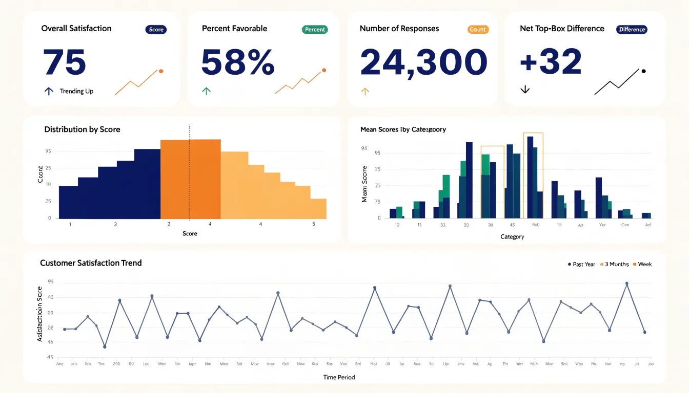
Beneath the KPI row, arrange the chart breakdowns in a logical hierarchy:
- A diverging stacked bar chart showing the distribution of responses across every survey item, with a vertical reference line marking the midpoint.
- A ranked bar chart of mean scores by category showing which areas lead and which lag.
- A line or column chart tracking scores over time to add context.
Group related visualizations into panels with clear headers, and align them on a consistent grid so the eye travels naturally from summary to detail.
Interactivity unifies these elements into a cohesive reporting tool. Add filter controls for demographic segments, survey waves, or question groups, and connect them so every card and chart updates together from a single selection. Use hover tooltips to reveal exact counts and percentages without cluttering the static view, and allow clicking a bar or KPI card to drill down into the underlying item detail. Maintain a consistent color palette across every view so the dashboard reads as a single artifact rather than a collection of unrelated charts.
Frequently Asked Questions
What is a diverging bar chart used for in Likert scale surveys?
A diverging bar chart arranges each survey item as a horizontal bar split around a central axis, with agreement responses extending one direction and disagreement the other. It lets readers compare the balance of sentiment across many items without reorienting at each row.
How do I build a 100 percent stacked bar chart for Likert scale data?
Convert raw counts into percentages within each question, order the segments consistently across all bars, and assign distinct colors to each rating point. Label segments with percentage values and note the base number where sample sizes differ.
What colors work best for Likert scale charts?
Use sequential palettes that move from light to dark within one hue, or divergent palettes with two contrasting hues and a pale or neutral center. The article cautions that red-green combinations can be hard to distinguish for people with color vision deficiency, while palettes such as blue and orange or purple and yellow-green remain legible for most viewers with deuteranopia or protanopia.
How should neutral responses be displayed in a diverging bar chart?
Neutral responses can sit on the center baseline to keep the scale structurally intact, or be isolated into a separate band, gap, or dedicated column to emphasize positive versus negative sentiment. Apply the placement consistently across all items and document the choice in a legend or annotation.
Should I use the mean or median for Likert scale average scores?
A mean can describe overall tendency when responses are reasonably spread out and roughly symmetric, but the median is more reliable when responses cluster at one end or include extreme answers. The article recommends reporting the mean alongside the median and also reporting response frequencies or percentages.
How do I handle missing data when calculating Likert scale percentages?
Base each question’s percentage on the number of valid responses rather than the total sample size, and clearly label the base size in charts and tables. Distinguish item non-response from unit non-response and document your handling method consistently.
Tony Astor
Tony writes about data visualization and the tools people use to build charts and dashboards. More about Data Illustrator