How to Visualize Large Datasets Without Clutter
 By Tony Astor ·
How to Visualize Large Datasets Without Clutter
Use transparency (alpha 0.05–0.2), hexbin plots, heatmaps, binning, sampling, or clustering to reduce overplotting in large datasets, encoding density through color instead of individual marks. Pair these with progressive loading, semantic zoom, interactive filters, smart label placement, tooltips, perceptually uniform palettes, and minimal chart junk to keep dense visualizations legible and responsive.
Table of Contents
Scatter Plot with Transparency
A scatter plot with transparency addresses overplotting, where many data points occupy the same or nearby coordinates and merge into an opaque mass that obscures underlying patterns. By adjusting the alpha opacity of the markers, overlapping points accumulate visually: areas with many points become darker or more saturated, while sparser regions remain lighter. This technique encodes density through color intensity, making dense clusters, hotspots, and outliers apparent without separate aggregation steps.
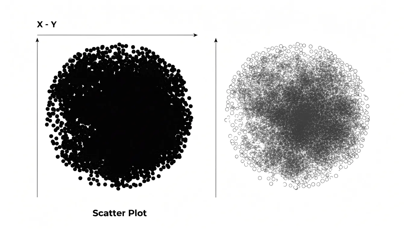
For large datasets, setting a low alpha value—typically between 0.05 and 0.2—ensures that even thousands of points remain distinguishable, as individual markers blend smoothly to form a continuous gradient. The result preserves the granularity of each observation while revealing the overall distribution. Because each point contributes to the final color, transparency also prevents points from being completely hidden by others. It is particularly useful in high-density coordinate charts where traditional scatter plots fail to convey data concentration.
Hexbin Plot
When data points number in the tens of thousands or more, a conventional scatter plot collapses into a solid smear. A hexbin plot addresses this by dividing the plotting area into a grid of regular hexagons and counting how many observations fall inside each cell. The result is a tessellated map in which every hexagon carries a single aggregate value, typically the count of points it contains, translated into color along a continuous gradient. Dense regions glow with saturated color while sparse regions recede into pale tones.
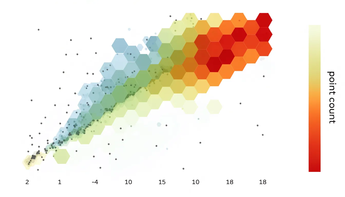
Hexagons earn their place for geometric reasons. Among regular shapes that tile a plane without gaps, hexagons sit closest to a circle, so each bin samples its neighborhood with less directional bias than a square grid would introduce. The six-sided tiling also avoids the visually distracting alignment of cells along horizontal and vertical axes that square bins can create, so gradients and clusters appear smoother and more organic.
By substituting counts for individual marks, the hexbin plot trades exact positional information for an honest summary of local density, keeping rendering costs manageable regardless of dataset size. Analysts typically pair the plot with a colorbar so the count scale stays explicit, and they tune the grid size to balance resolution against noise. Too few hexagons obscure fine structure; too many reintroduce the sparseness of the original scatter. Chosen well, a hexbin plot reveals hotspots, ridges, and empty zones that a dense cloud of points would otherwise conceal.
Heatmap
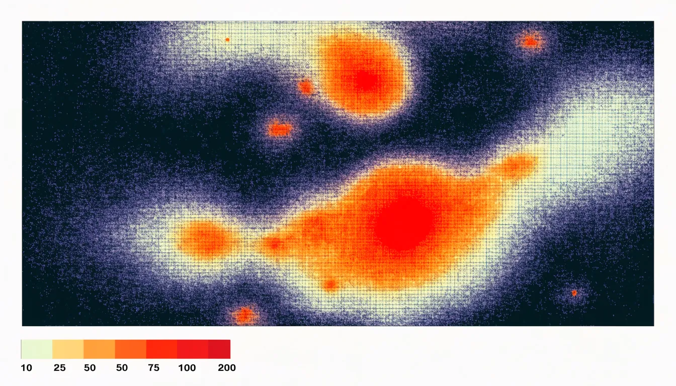
Like a hexbin plot, a heatmap summarizes points rather than drawing each one. The plotting area is divided into a grid of cells, typically rectangles or hexagons, and every data point is assigned to the bin that contains it. Each cell is then shaded according to how many points it holds, transforming a cloud of markers into a smooth field of color that reveals where observations concentrate.
The choice of bin size and grid shape sets the resolution of the summary. Finer bins preserve local detail and expose small clusters, while coarser bins smooth away noise and emphasize broad regional structure. Once points are aggregated, a gradient color scale maps counts to hue or luminance. Sequential palettes, running from light to dark or pale to saturated, work well for single-peaked distributions.
Binning solves the overlap problem structurally. Every point counts exactly once, so dense cores remain visible alongside thin peripheral regions, and the total density across the map stays faithful to the data. Hot spots, gradients, boundaries, and empty zones emerge as shapes rather than as accumulations of individual marks, making heatmaps a dependable default for spatial exploration of very large point collections.
Data Aggregation
Data aggregation combines individual data points into larger groups or bins, reducing the number of visual marks while preserving overall trends. Techniques such as mathematical binning, rolling averages, and statistical summaries reveal the big picture by summarizing data at a higher level:
- Mathematical binning divides the data range into intervals, or bins, and calculates a summary statistic for each bin, such as the count, mean, or sum of points within it. This approach is used for creating histograms or heatmaps, where point density is represented by height or color. Choosing appropriate bin sizes highlights trends without losing the overall shape of the distribution.
- Rolling averages smooth out short-term fluctuations and highlight longer-term trends. This technique calculates the average of a fixed number of consecutive data points and moves the window across the dataset. It is commonly used in time series analysis to reduce noise and make patterns—such as seasonal variations or gradual changes over time—more visible.
- Statistical summaries, such as median, quartiles, or standard deviation, provide a concise description of the data distribution. These summaries can be visualized using box plots or error bars, which convey spread and central tendency without plotting every point. This is especially helpful when comparing multiple groups or categories.
The key is to choose a level of aggregation that balances detail with clarity, keeping the visualization informative and interpretable.
Sampling
When a dataset contains millions of records, plotting every point often overwhelms both the rendering engine and the reader. Instead of drawing the full dataset, sampling draws a representative subset that still communicates the underlying pattern.
Random sampling is the simplest approach. Each point has an equal chance of being selected, so a random draw of, say, ten thousand points from a million will generally reproduce the broad shape of the distribution, including the density of clusters and the spread of outliers. This method is fast to implement and requires little knowledge of the data’s structure.
Stratified sampling refines the idea by dividing the dataset into meaningful groups—such as categories, time bands, or regions—and drawing a proportional sample from each one. This matters when certain segments are small but analytically important; a purely random draw might underrepresent or miss them entirely, while stratified sampling guarantees that every segment retains its correct share of the visual.
Rendering fewer points reduces draw time and keeps interactions like zooming, panning, and filtering responsive. Integrity is preserved as long as the sample is drawn correctly and documented, with the sample size chosen large enough to stabilize the pattern and small enough to keep the plot legible. Readers should be told that sampling was used, and tools should offer a way to inspect the full data on demand.
Clustering
Clustering transforms thousands of individual data points into a smaller set of meaningful groups. When a dataset contains dense regions where points overlap, a clustering algorithm can identify these concentrations and represent them with a single marker, such as a centroid, or with a boundary that defines the group’s extent.
Two widely used algorithms for this purpose are k-means and DBSCAN:
- K-means partitions the data into a pre-specified number of clusters by iteratively assigning each point to the nearest centroid and recalculating the centroids based on the assigned points. The result is a set of compact, roughly equal-sized clusters summarized by their centroids. This approach works well when data naturally forms spherical groups and when the analyst has a reasonable estimate of the number of clusters.
- DBSCAN groups points that are closely packed together while marking points in low-density regions as outliers. It does not require the number of clusters to be specified in advance and can discover clusters of arbitrary shape, making it suitable for datasets with irregular spatial structures and noise.
Once clusters are formed, the visualization can display each cluster as a centroid with a size or color that encodes the number of underlying data points, or as a shaded region that conveys the group’s spatial extent. Both representations serve as a preprocessing step to create readable visual summaries of large datasets.
Small Multiples
Small multiples divide a dense or multivariate graphic into a grid of small, simple charts that share the same axes, scales, and visual encoding. Each panel shows one slice of the data—such as a single category, region, or time period—while the overall grid preserves the relationships between those slices at a glance. Because every panel uses identical scales and marks, viewers can scan across the grid and compare patterns directly without recalibrating what a taller bar or darker shade means from one chart to the next.
This approach is especially useful for high-density or multivariate data, where placing every series on a single canvas produces overlapping lines, crowded legends, and ambiguous points. Splitting the data into a grid keeps each panel readable while the arrangement communicates the big picture. A viewer can spot which categories follow a similar trajectory, where an outlier sits apart from the rest, and how a seasonal or geographic pattern repeats across panels. Synchronized axes also allow subtle contrasts to emerge, since a small change in one panel stands out against the steadier background of the others.
The grid works best when panels are genuinely simple, with a clear title or label for each and a minimal set of reference lines. Consistent ordering—whether alphabetical, by value, or by trend—helps the eye move through the grid in a predictable way and makes differences between panels easier to notice. Compact panels with shared legends and axis labels reduce repetition and free space for the data itself.
Progressive Loading
Progressive loading reveals detail in proportion to the viewer’s current focus. Level-of-detail techniques maintain multiple representations of the same data, each tuned to a particular zoom range. At the full extent, the map or chart draws an aggregated summary: clustered points, binned densities, or simplified geometries that convey the overall shape of the data without exposing individual records. As the viewer zooms in, the system swaps these coarse representations for finer ones, eventually resolving to raw data points at the deepest levels.
Implementation typically involves a spatial index, such as a quadtree or an R-tree, that organizes features by geographic or coordinate extent. Each node in the index stores a precomputed summary, so the renderer only fetches the tiles or records intersecting the current viewport at the current zoom. Requests are issued on demand, which means the initial payload stays small and the visualization becomes interactive almost immediately. Subsequent detail streams in as needed, often with transitional placeholders to keep the experience smooth.
This approach improves both performance and clarity. The browser or rendering engine processes a bounded number of features per frame, regardless of total dataset size, while granular data appears only where the viewer has signaled interest through zooming. The visualization scales gracefully from a continental overview down to individual observations, presenting the detail that remains legible at each scale.
Zoom and Focus Controls
Zoom and focus controls let users move deliberately between the broad shape of a dataset and the fine grain of individual records. Semantic zooming is central to this experience. When a user zooms in on a dense scatter plot or a crowded timeline, the display changes what it shows rather than simply magnifying pixels. Labels may appear only once marks are large enough to separate, clusters may split into their constituent points, and summary shapes may resolve into the underlying values. The overview communicates distribution and trend, while the close view communicates exact position and identity.
Overview-plus-detail views complement semantic zooming by keeping a miniature of the full dataset visible alongside the focused region. A small map, a compressed timeline, or a thumbnail of the whole chart acts as a persistent anchor, showing where the current viewport sits and what lies outside it. Users can drag a viewport rectangle across the overview to navigate, or click a cluster to jump directly into it, without losing their sense of position.
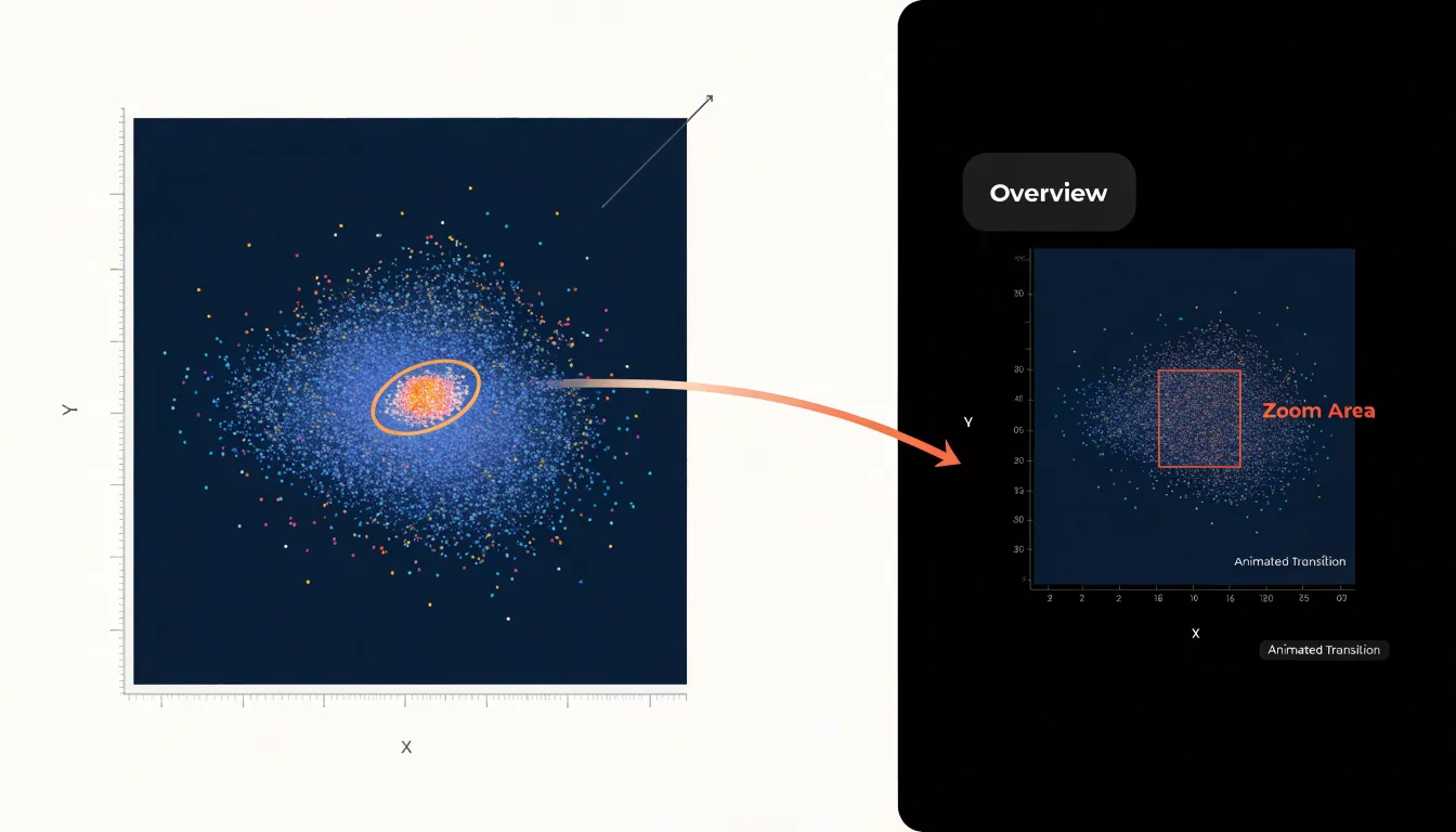
This combination matters because zooming in isolation tends to strip away context: a user who magnifies a single point often cannot tell whether that point is typical or unusual within the larger population. With an overview panel present, the focused detail remains situated within the whole. Smooth, animated transitions rather than instantaneous jumps help users track what changed between views. Controls should also offer clear escape routes, such as a reset button or breadcrumb trail, so exploration feels reversible and low-risk.
Interactive Filtering
Interactive filtering gives viewers direct control over which data points remain visible at any moment. Rather than presenting a single static view that attempts to show everything at once, the visualization offers controls that let users narrow the dataset to the subset relevant to their current question:
- Faceted filters use checkboxes or toggle buttons tied to categorical dimensions, such as region, product type, or status, letting users switch entire groups of points on and off. When a viewer deselects three of eight regions, hundreds of overlapping marks disappear, and the remaining patterns become legible. Facets work best when categories are mutually exclusive and the number of options stays manageable, so the filter panel itself does not become a source of clutter.
- Range sliders handle continuous dimensions. A viewer can drag endpoints along a timeline, price bracket, or measurement scale to isolate a band of interest. Dual-handle sliders show the selected window while excluded data fades away. Sliders pair naturally with brushing interactions on the chart itself, where dragging across a region of the plot filters other linked views.
- Dynamic queries tie these controls together through direct manipulation. Each change to a filter re-renders the display immediately, giving instant feedback that supports exploration. Users can test hypotheses, compare subgroups, and drill into dense clusters without navigating away from the chart.
Smart Label Placement
Smart label placement decides where each text annotation should sit so it communicates its value without competing with neighboring labels or obscuring the marks beneath it. In a dense visualization, hundreds of labels may be candidates for display, yet only a fraction can appear at once before the chart becomes illegible.
The core technique for managing this is collision detection: before a label is drawn, the rendering system calculates its bounding box and tests it against the boxes of labels already placed, as well as against key data marks and boundaries. If an overlap is detected, the label is nudged to an alternative position, shortened, or deferred to a later pass. Efficient implementations often use spatial indexing structures, such as quadtrees or grid buckets, so each candidate is compared against a small local set of neighbors rather than every other label on the canvas. This keeps computation tractable even when the dataset contains thousands of points.
While collision detection determines what cannot be shown, prioritized labeling strategies determine what should be shown first. Each label is assigned a priority derived from attributes such as magnitude, recency, or category importance, and the algorithm attempts placement in descending order. The most significant annotations claim their preferred positions, while lower-priority labels are placed afterward on a best-effort basis and may be omitted entirely when space runs out. A related refinement is the try-list approach, in which each label carries an ordered set of candidate positions, typically beginning directly above the mark and rotating through offsets to the right, below, and left. The algorithm walks this list and accepts the first position that passes the collision test.
Tooltips
Tooltips manage visual complexity by deferring secondary information until the user actively seeks it. By offloading secondary metrics and granular data points to hover cards, you preserve the clarity of the main canvas while keeping detailed information within easy reach. When a user hovers over a data point, a tooltip can reveal precise values, additional dimensions, or contextual explanations that would otherwise overcrowd the display.
For example, a line chart showing trends over time can display just the lines and axes, with tooltips providing exact values, percentage changes, or related metrics for each point. Similarly, scatter plots can use tooltips to show labels for individual points without permanent text that would overlap and obscure patterns. Tooltips should be informative yet concise, with clear formatting and intuitive placement, enhancing understanding without requiring extra clicks or navigation.
Color Palettes
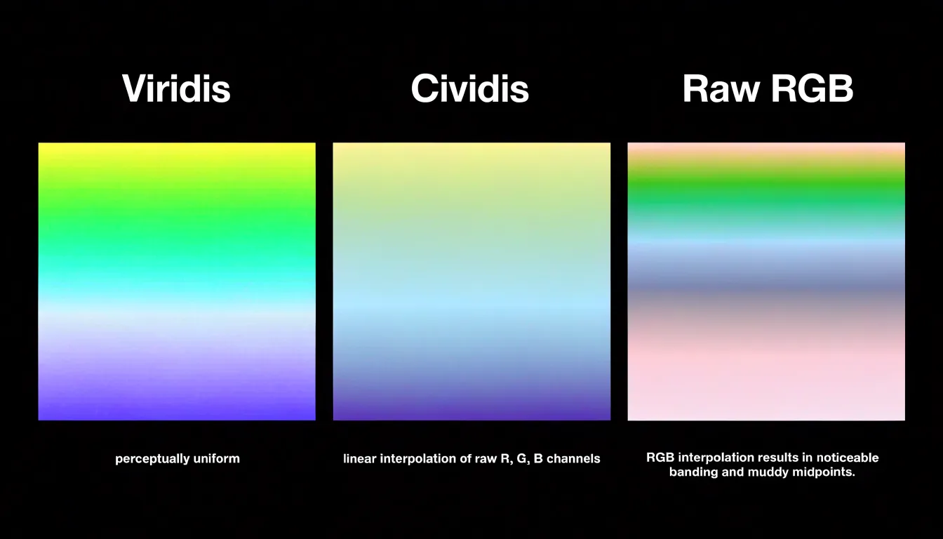
When thousands of points or cells compete for space, a well-chosen palette lets viewers read density and value at a glance. The foundation of that clarity is the perceptual uniformity of the color scale. A perceptually uniform sequential scale, such as Viridis or Cividis, changes in lightness and hue at a steady rate across its range, so equal steps in the data appear as equal steps in visual difference. Scales built on raw RGB interpolation create uneven jumps, banding, and muddy midpoints that distort how viewers judge magnitude. A uniform scale keeps the mapping honest and remains readable for viewers with color vision deficiencies.
For data that pivots around a meaningful midpoint, such as a zero baseline or an average, diverging scales serve the same purpose on two axes. A careful diverging palette moves from a cool, dark low end through a neutral light center to a warm, dark high end, with symmetric lightness so that values above and below the midpoint register with comparable strength. This symmetry makes departures in either direction legible and prevents one side of the scale from visually dominating the other.
Restraint also applies to how many colors the eye must process at once: limit the palette to a small set of steps, reserve saturated or warm tones for values that deserve attention, and let low values recede into calm, muted shades.
Chart Junk Removal
Gridlines and borders are common culprits of visual clutter because they add ink without adding information. When a chart is dense with data points, these structural elements compete for attention. The solution is to remove any line, box, or shading that does not directly encode data or guide interpretation.
Start with the chart’s frame. A full border around the plot area often serves no purpose beyond decoration; removing the top and right borders, or eliminating the border entirely, opens up the chart and reduces visual noise. Next, evaluate gridlines. Horizontal gridlines can help with reading values, but they should be thin, light gray, and sparse. Vertical gridlines are rarely needed unless the x-axis represents a continuous scale where precise alignment matters. In many cases, you can replace gridlines with direct labeling or subtle tick marks.
The goal is to maximize the data-ink ratio, a concept introduced by Edward Tufte, which advocates for using ink only to present data. Stripping away non-essential elements makes the data itself more prominent and improves accessibility, as viewers with cognitive or visual impairments can process the chart more easily. Removal should be thoughtful and iterative: test the chart with and without each element, keeping what aids comprehension—such as axis labels and a subtle baseline—and removing what does not.
Dashboard Layout
When multiple charts share a single interface, each element competes for attention. Giving every visual breathing space begins with treating whitespace as an active design material rather than leftover room. Generous margins around charts, consistent gutters between panels, and clear separation between distinct analytical themes allow the eye to rest and reset as it moves across the dashboard.
Visual hierarchy complements spacing by guiding attention in a deliberate order. The most important metric or trend should occupy a prominent position—typically the top-left region for left-to-right reading cultures—and receive the largest allocation of canvas. Secondary charts sit below or beside it at reduced scale, while supporting detail recedes into smaller components or secondary tabs. This ordering lets viewers absorb the headline insight first and then drill into context.
Balanced component sizing keeps the layout coherent. Charts of similar analytical weight should share comparable dimensions, while a single oversized chart signals priority and a grid of small multiples signals comparison across categories. Uneven sizing without clear intent creates visual noise, so alignment to an underlying grid helps every panel feel anchored. Consistent card sizes, aligned axes, and repeated spacing values produce a predictable structure that reduces cognitive load.
Frequently Asked Questions
How do I make a scatter plot with thousands of points less cluttered?
Use transparency by adjusting the alpha opacity of the markers. For large datasets, a low alpha value—typically between 0.05 and 0.2—lets overlapping points accumulate visually so dense areas become darker or more saturated while individual points remain distinguishable.
When should I use a hexbin plot instead of a scatter plot?
A hexbin plot is useful when data points number in the tens of thousands or more, because a conventional scatter plot can collapse into a solid smear. It divides the plotting area into hexagons, counts how many observations fall inside each cell, and translates those counts into color along a continuous gradient.
How does a heatmap show where large numbers of points are concentrated?
A heatmap divides the plotting area into a grid of cells, assigns every data point to the bin that contains it, and shades each cell according to how many points it holds. This transforms a cloud of markers into a smooth field of color that reveals where observations concentrate.
What is the difference between random sampling and stratified sampling?
Random sampling gives each point an equal chance of being selected, so a random draw can reproduce the broad shape of a distribution. Stratified sampling divides the dataset into meaningful groups and draws a proportional sample from each one, which helps small but analytically important segments retain their correct share of the visual.
What is the difference between k-means and DBSCAN for clustering large datasets?
K-means partitions data into a pre-specified number of clusters by assigning each point to the nearest centroid and recalculating centroids, working well for compact, roughly equal-sized, spherical groups. DBSCAN groups closely packed points, marks points in low-density regions as outliers, does not require the number of clusters to be specified in advance, and can discover clusters of arbitrary shape.
How can tooltips help reduce clutter in dense visualizations?
Tooltips defer secondary information until the user hovers over a data point, preserving the clarity of the main canvas while keeping detailed information within easy reach. They can reveal precise values, additional dimensions, or contextual explanations without permanently crowding the display.
Tony Astor
Tony writes about data visualization and the tools people use to build charts and dashboards. More about Data Illustrator