How to Visualize Geographic Data: Map Types Explained
 By Tony Astor ·

How to Visualize Geographic Data
Geographic data is visualized by matching the data type to a map style: choropleth maps for rates by region, proportional symbol maps for raw counts at points, dot density and heat maps for concentration, contour maps for continuous fields, cartograms for data-weighted areas, flow maps for movement, and bivariate maps for two variables at once.
Table of Contents
Choropleth Maps
A choropleth map divides a geographic area into predefined regions, such as states, counties, or countries, and fills each region with a color drawn from a gradient corresponding to a numeric variable. Lighter shades typically represent lower values and darker shades higher values, so a reader can immediately see where a measure clusters, spikes, or thins out. This makes choropleth maps especially effective for standardized data—figures adjusted to account for differences in area or population. Population density is the classic example: raw population counts would simply highlight large regions, while residents per square mile reveals genuine concentration. Literacy rates, unemployment percentages, median income, and vaccination coverage follow the same logic, expressing a quantity as a proportion or rate so that regions of very different sizes can be compared fairly.
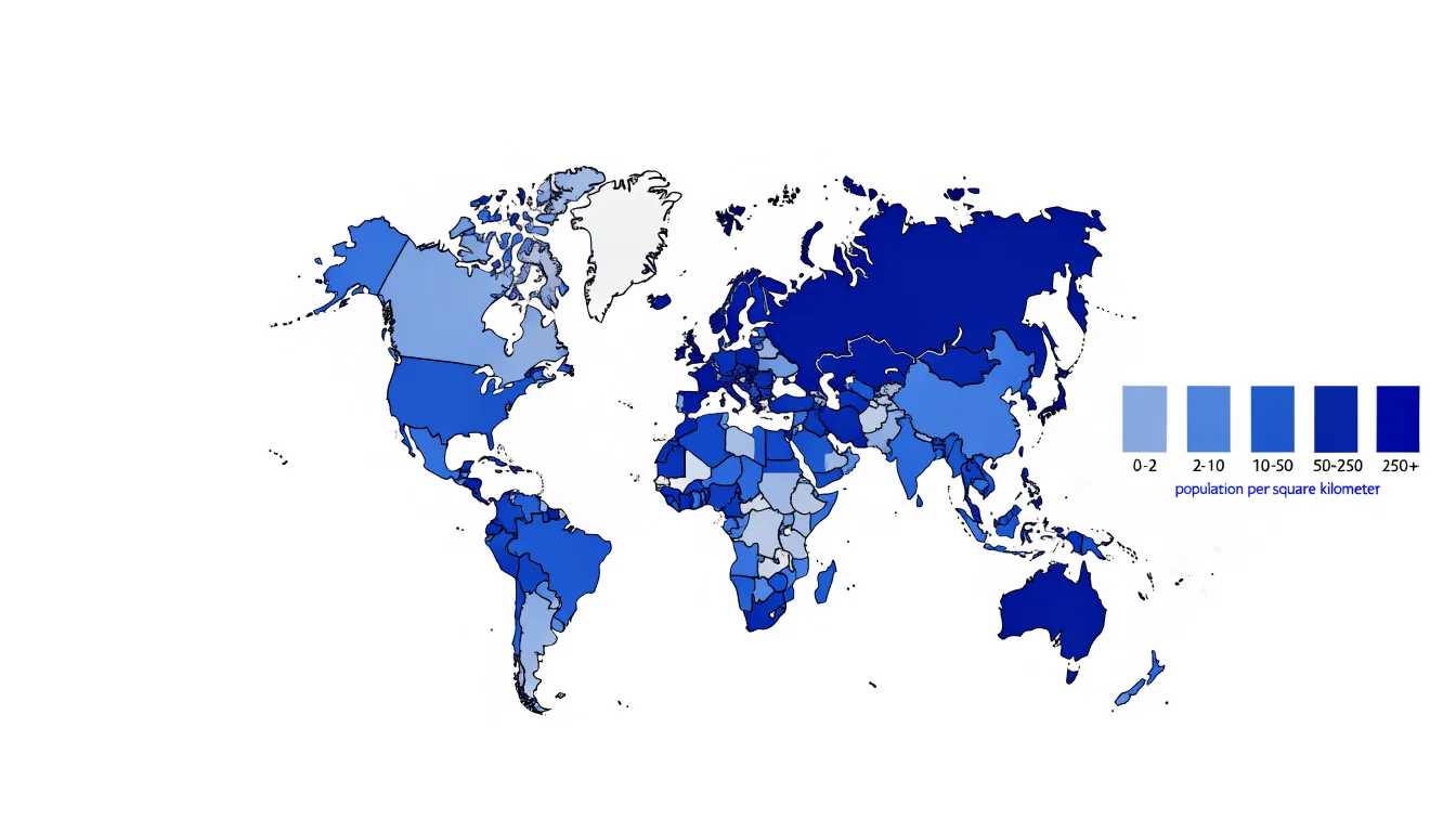
Building a choropleth map starts with joining a table of values to a shapefile or GeoJSON boundary file, matching records through a shared identifier such as a state code or country name. Once joined, a color scale is chosen and the numeric range is divided into classes. Common classification schemes include equal intervals, quantiles, and natural breaks, and the choice of scheme strongly influences which patterns appear prominent. Designers select an appropriate sequential palette, using a single hue that darkens with magnitude so the visual ordering matches the numeric ordering. Legends should display the class breaks explicitly, allowing readers to translate color back into value. Because the eye naturally compares shaded areas, choropleth maps excel at revealing regional disparities across many administrative units at once, from neighborhood-level census tracts to national boundaries.
Proportional Symbol Maps
Proportional symbol maps place a scalable shape at each location on a basemap, with the size of that shape tied directly to the value it represents. Circles are the most common choice, though squares, triangles, and icons such as people or buildings also work well when the subject calls for them. Larger symbols indicate larger totals and smaller symbols indicate smaller totals. Because the symbols float above the basemap rather than recoloring the regions beneath them, the underlying geography remains fully visible and undistorted. Coastlines, borders, roads, and city footprints stay intact, making this technique well suited to displaying raw counts such as population totals, sales figures, incident reports, or the number of facilities in a region.
Sizing the symbols requires care. Area, rather than diameter, should scale in proportion to the value, since readers naturally judge the magnitude of a shape by how much space it covers. A circle representing twice the value of another should have twice the area, which means its radius grows by the square root of two. Scaling the radius directly to the value produces symbols that look dramatically larger than they should and exaggerates differences between locations. Designers often add a legend with two or three reference circles and their exact values so readers can estimate quantities accurately.
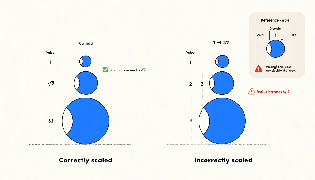
Proportional symbols handle overlapping points through transparency, outlines, or slight offsets. This technique works best with data tied to specific point locations, where totals can be anchored to a recognizable place and compared across the map at a glance.
Dot Density Maps
A dot density map represents geographic data by scattering uniform dots across a map, with each dot standing for a fixed quantity of whatever is being measured, such as one person, one household, or one incident. Because every dot carries the same value, viewers can read concentration directly from the visual weight of the pattern. A dense thicket of dots signals a crowded area, while broad stretches of empty space show sparse settlement. The eye grasps this contrast instantly, without consulting a legend or decoding a color ramp.
Building a dot density map begins with counts tied to geographic units, such as census tracts or districts. Each unit’s total is divided by the value assigned to a single dot, and that many dots are placed randomly or semi-randomly within the unit’s boundaries. Random placement avoids the false precision of marking exact locations while preserving the overall distribution across space. The result is a texture of points that mirrors how people or events cluster on the ground.
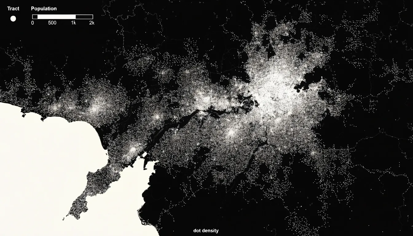
This approach shines when the goal is to reveal spatial distribution and population shifts across regions. Comparing dot patterns from two time periods, for example, makes it possible to see where growth has tightened into dense clusters and where populations have thinned out. Urban cores, suburban fringes, and rural expanses each take on a distinct visual character. The uniform dot size keeps attention on density rather than magnitude, communicating how evenly or unevenly a phenomenon spreads across a territory.
The technique does carry tradeoffs. Because dots are distributed within larger units, the map is most honest at regional and national scales and less reliable for street-level questions. Dot color and size should stay consistent so the density signal remains clear.
Heat Maps
Instead of pinning thousands of individual points onto a map—which quickly turns into an unreadable cluster of overlapping markers—a heat map aggregates those locations into a continuous surface. Each location contributes weight to the pixels or grid cells around it, and adjacent contributions accumulate. The result is a smooth color gradient in which warmer or more saturated tones mark areas of concentrated activity and paler tones recede into low-density regions. This approach works especially well for phenomena that occur at very fine granularity, such as website sessions tied to IP-derived locations, emergency call records, or reported crime incidents spread across a city.
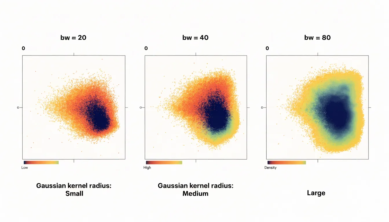
Building an effective heat map begins with choosing a kernel and a radius that control how far each point’s influence spreads. A small radius reveals tight, local clusters but can fragment the picture; a larger radius smooths the surface and emphasizes broad regional patterns. Analysts often test several settings before settling on one that matches the scale of the question at hand. Sequential palettes that progress from light to dark, or through a single hue family, are the most legible for representing a single density dimension, while rainbow scales tend to introduce false boundaries that readers interpret as real thresholds.
Heat maps also carry a responsibility toward interpretation. Because they generalize, a bright patch can reflect many events in a small area as easily as a few events with wide spreading kernels, so legend design and an explicit statement of the bandwidth help audiences read the map correctly. Used thoughtfully, heat maps point decision-makers toward the neighborhoods, corridors, or time periods where attention is most needed.
Isarithmic Contour Maps
Isarithmic contour maps visualize continuous geographic phenomena by drawing lines—called isarithms or contours—that connect points of equal quantitative measurement across a surface. An elevation map uses contour lines to link points at the same height above sea level, a temperature map connects points with identical average temperatures, and a rainfall map joins locations receiving the same amount of precipitation. The result is a set of nested lines that reveal the shape and gradient of the phenomenon: where lines are close together, values change rapidly; where they are far apart, the change is gradual. This makes isarithmic maps particularly effective for showing continuous fields such as topography, climate, and atmospheric pressure.
The process begins with a set of sample points, each with a measured value. The mapmaker selects a series of intervals—for instance, every 100 meters of elevation or every 5 degrees of temperature—and interpolates between the points to estimate where each contour line should fall. The lines are then drawn to connect points of equal value, forming a visual surface that can be read like a topographic sheet. To enhance interpretation, the spaces between contours are often filled with color gradients, creating a choropleth-like effect that emphasizes highs and lows and helps viewers quickly identify peaks, valleys, ridges, and depressions.
Isarithmic contour maps are used across many fields: meteorologists rely on isobars to show pressure systems, geologists use structure contours to map subsurface layers, and hydrologists employ isohyets to depict rainfall distribution. The technique can represent any continuous variable that varies smoothly over space, though it requires careful interpolation and a sufficient density of data points to avoid misleading artifacts.
Cartograms
A cartogram is a map that deliberately distorts geographic space to convey information about a variable other than land area. Instead of keeping regions fixed by their physical boundaries, a cartogram resizes them according to a chosen variable, such as population, GDP, or election results. This transformation allows viewers to see patterns that might be obscured when land area dominates the visual field.
There are two main types of cartograms: contiguous and non-contiguous. In a contiguous cartogram, the overall shape of the map is preserved as much as possible while regions are warped and stretched to achieve the desired area proportions. This maintains the familiar outline of a country or continent, making it easier for viewers to recognize the geography, though extreme distortion can make small regions difficult to locate. In a non-contiguous cartogram, each region is scaled independently and placed in its approximate geographic location, often resulting in a collection of floating shapes. This preserves the shape of individual regions but sacrifices overall geographic continuity.
Population cartograms are common because they reveal true demographic weight, highlighting densely populated regions that appear small on a standard map. GDP cartograms show economic output, drawing attention to wealthy regions regardless of physical size. Election cartograms display voting patterns without the bias of land area, where large, sparsely populated areas might otherwise dominate the visual narrative.
Creating a cartogram requires specialized algorithms that balance accurate area representation with recognizability, enabling viewers to see the world in proportion to the data rather than to the land.
Flow Maps
Flow maps trace movement between places using vector lines and arrows to represent the volume, direction, and origin-destination routes of phenomena such as goods, migrants, or digital traffic. Each line connects an origin point to a destination, and the width of the line typically scales with the volume of flow, allowing viewers to quickly grasp which connections are most significant. Arrows indicate whether a flow is one-way or bidirectional.
Flow maps are particularly effective for revealing spatial patterns of interaction. A flow map of global shipping routes can highlight major trade corridors, a map of migration flows can show population movements between regions, and a map of digital traffic can visualize data transfers between server locations to show network dependencies. By showing both the magnitude and the geography of movement in a single view, flow maps allow viewers to identify dominant pathways, bottlenecks, and asymmetries in exchange.
Creating effective flow maps requires careful design:
- Line width must scale proportionally to flow volume, though extreme values can cause clutter and may require normalization or logarithmic scaling.
- Directional arrows should be clear without overwhelming the map.
- Curved lines are often used instead of straight lines to reduce overlap and suggest organic movement.
- Color can differentiate types of flow or highlight specific routes.
- Interactive features like filtering or zooming help manage complexity when many flows exist.
Bivariate Color Maps
Bivariate color maps display two variables on a single map through the intersection of two distinct color scales. Each variable is assigned its own sequential ramp, and the two ramps are combined into a grid—usually three by three—producing nine unique color classes in the legend. Every polygon or region on the map receives a color that encodes both values at once. For example, one axis might run from low to high population density while the other runs from low to high median income. A dark blue corner of the grid can signal places where both variables are high, a pale corner can mark places where both are low, and the mixed hues along the diagonal or in opposite corners reveal combinations such as dense, low-income areas or sparse, high-income ones.
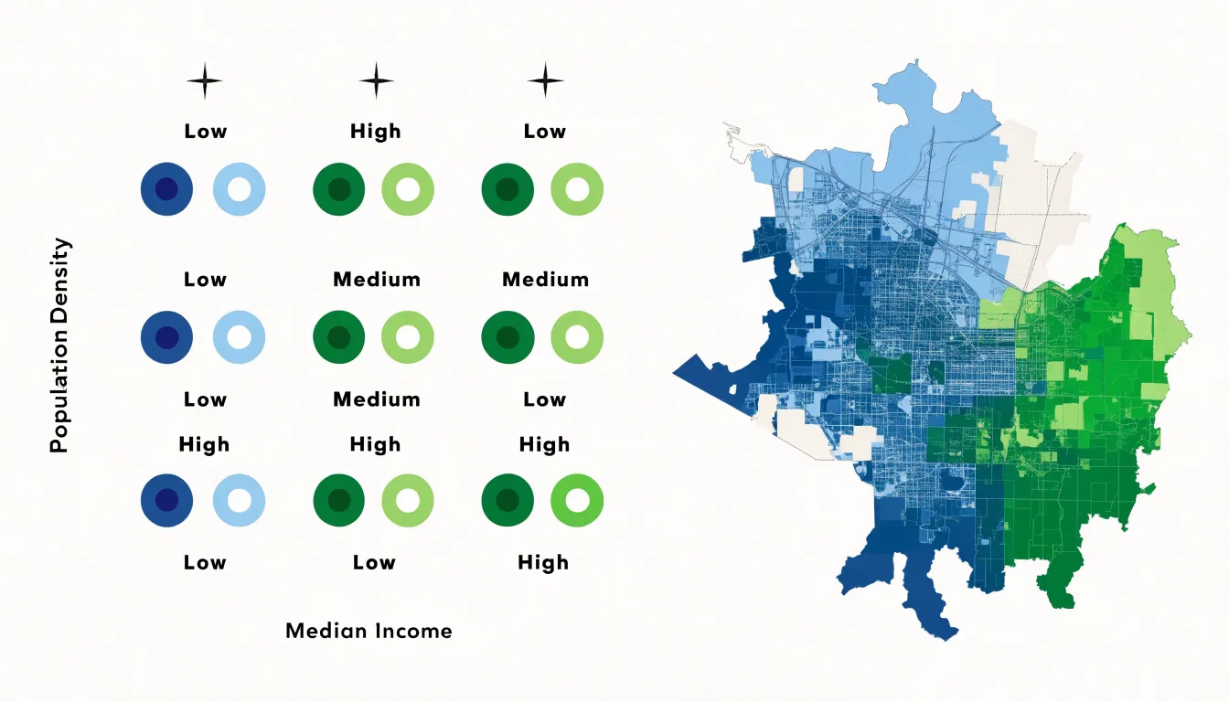
The main strength of this approach lies in the relationships it makes visible. When colors cluster along a diagonal in the legend, the two metrics tend to correlate across space. When the map fills with colors from mismatched corners, the variables appear to move independently or inversely. Readers can spot spatial patterns that would be difficult to detect in two separate choropleth maps viewed side by side, because the bivariate version keeps every location in a single visual field.
The format demands care. Legends must be clear and labeled, since readers need to learn a two-dimensional key rather than a simple ramp. Too many classes can overwhelm the eye, so three-by-three grids remain the most practical choice for most projects. Colors should also remain distinguishable when printed in grayscale or viewed by readers with color vision deficiencies.
Hexagonal Binning Maps
When a dataset contains thousands of individual points, a hexbin map prevents overlapping markers by aggregating points into a grid of regular hexagons, with each cell shaded to represent the count or aggregated value of the observations falling within it. This reduces visual clutter while preserving the underlying spatial distribution across neighborhoods, regions, and countries.
A hexagonal grid offers distinct geometric advantages. Hexagons tile a plane without gaps and share edges with six neighbors instead of four, giving each cell more evenly distributed proximity to adjacent cells than a square grid provides. This reduces the directional distortion of square bins, where distances to diagonal neighbors differ noticeably from distances to lateral ones, resulting in a more uniform sense of spacing and smoother visual transitions between categories.
Equally important, hexagons sidestep the distortions of administrative boundaries. Political and census units vary wildly in size and shape—urban districts may be tiny and densely packed while rural counties sprawl across vast areas—which can mislead on choropleth maps when large, sparsely populated regions dominate the visual field. Because uniform hexagons are defined by the data analyst rather than by historical or political circumstances, each cell covers a comparable geographic area. Color intensity reflects the actual concentration of observations rather than the arbitrary size of a jurisdiction, making regional comparisons fairer and less susceptible to border-driven bias.
Hexbin maps suit any dataset with meaningful point-level coordinates, including incident reports, customer locations, sensor readings, and demographic records. Analysts control cell size and resolution, allowing them to zoom from national overviews to local detail while maintaining the same visual grammar.
Network Maps
Network maps represent systems as a set of nodes (individual elements) and edges (the relationships connecting them). In a geographic network map, nodes are placed at their real-world locations while edges trace the links between them, reflecting both the physical arrangement of the system and its internal connectivity. This dual character makes network maps useful for understanding infrastructures whose behavior depends on how their parts are joined together.
- Flight routes: Airports are nodes and direct connections are edges, revealing hubs where many routes converge, heavy-traffic corridors, and peripheral locations served by a single link.
- Power grids: Generating stations, substations, and load centers are nodes while transmission lines are edges, showing which parts of the network are densely interconnected and which depend on a few critical links.
- Supply chains: Suppliers, factories, warehouses, and distribution centers serve as nodes connected by shipping lanes or trucking routes.
- Logical infrastructures: Internet backbone connections or financial transfers between institutions place nodes at physical locations while edges describe flows of data or capital.
The visual vocabulary of nodes and edges scales well to complex systems. Node size can encode volume, edge thickness can encode capacity or frequency, and color can distinguish connection types, revealing structure, bottlenecks, and dependencies that are difficult to perceive from a table of routes.
Interactive Maps
Interactive maps transform a static picture into a workspace for exploration. At the most basic level, zoom levels let users move between a regional overview and the fine detail of a single neighborhood. Information can adapt as the map scales, so a country view might display aggregate totals while a street-level view reveals individual locations, keeping the map readable at every scale.
Tooltips and hover states add a second layer of engagement by surfacing details on demand. Moving a pointer over a marker or region can trigger a small popup with exact values, labels, or short descriptions without cluttering the base map. Clicking can open richer panels with charts, images, or related records, letting users drill into particular points.
Dynamic filtering turns these maps into tools for customized discovery. Sliders, checkboxes, or dropdown menus let users narrow the data by category, date range, or threshold, redrawing the map immediately. A viewer can isolate a single product line or time period and compare its patterns against the whole. Together with zoom and hover states, filtering supports open-ended investigation through direct manipulation of the data.
Map Projections
Because a spherical Earth cannot be unrolled onto a flat sheet without stretching, tearing, or compressing parts of its surface, every flat map involves distortion. The craft of map projection is about deciding which distortions are acceptable for a given purpose across four spatial properties: area, shape, distance, and direction. A projection can preserve one or two of these faithfully, but geometric constraints prevent preserving all four at once.
- Equal-area projections preserve area, keeping every region in correct proportion to every other. This makes them valuable for thematic maps showing density or distribution, such as population or land cover, though shapes become stretched and skewed toward the map’s edges.
- Conformal projections preserve shape, keeping local angles and outlines accurate for navigation and reference maps. The trade-off is that area inflates dramatically at high latitudes, which is why Greenland appears enormous on some world maps.
- Other projections prioritize consistent distance from a central point or accurate compass bearings for specific analytical needs.
Designers should choose a projection deliberately, guided by the question the map is meant to answer. Comparing the land area of countries calls for an equal-area projection, while tracing shipping routes favors one that preserves direction. Documenting the projection in a caption or legend helps readers interpret what they see.
Map Colors
Selecting a color palette begins with matching the palette type to the nature of the data:
- Sequential schemes move from light to dark through a single hue and suit quantities that progress in one direction, such as population density or rainfall totals.
- Diverging schemes place two contrasting hues at either end of a neutral midpoint, working best for values that pivot around a meaningful center, like temperature anomalies or budget surpluses and deficits.
- Categorical schemes use distinct hues of similar visual weight to separate unordered groups, such as land-use types or political regions, where no category outranks another.
Accessibility deserves attention from the start. Roughly one in twelve men and one in two hundred women experience some form of color vision deficiency, most commonly red-green confusion. Palettes that lean on red versus green, or that separate categories only by hue, become unreadable for these viewers. Tools such as ColorBrewer and Coblis simulate how a palette appears under different types of color blindness so designers can test choices before publishing. Pairing hue with variation in lightness or saturation gives every reader a second channel for distinguishing values.
Legibility also depends on context. Because maps carry labels, boundaries, and basemap features, palettes need enough contrast against surrounding elements without overwhelming them. Sequential ramps should keep the lightest step clearly visible against the background, and categorical hues should sit at similar lightness so no category falsely appears more important. Limiting a palette to five to seven classes keeps differences perceptible, and testing the map at its final print or screen size confirms that distinctions survive real viewing conditions.
Matching Data to Map Types
Choosing a map style requires evaluating the data across three axes:
- Cardinality: Does each observation represent a discrete place, a line, or a surface? Point data (store locations, earthquake epicenters) calls for point symbols or dot density. Linear data (rivers, transit routes) suits line symbols. Areal data (census tracts, countries) fits choropleths, while continuous fields (temperature, elevation) demand isarithmic or heat map treatments. Mismatching cardinality and symbol type misleads viewers before a single color is chosen.
- Continuity: Phenomena that change abruptly at boundaries, such as political jurisdictions, should be mapped with crisp edges. Phenomena that vary smoothly across space require smooth interpolations or contour lines to preserve the gradient; representing them with hard-edged polygons implies false precision.
- Research question: Showing rankings or rates calls for a classed choropleth with a considered classification scheme. Identifying concentrations favors dot density or kernel density (heat maps), while questions about movement and interaction call for flow or network maps.
Evaluating cardinality, continuity, and purpose together rules out inappropriate styles early and ensures the map communicates the data’s structure accurately.
Dashboards
A map on its own answers where things are, but most analytical work requires understanding location alongside magnitude, trend, and category. Dashboards solve this by placing the map within a coordinated layout of complementary views: the map shows spatial distribution, a bar chart ranks regions by a chosen metric, a line chart tracks change over time, and KPI cards surface headline figures such as total revenue, average delivery time, or active sites. Together, they let a viewer move from geographic pattern to underlying cause without leaving the page.
Interaction connects these views. Filters—such as a date range selector, category dropdown, or region toggle—should propagate across every panel at once. Selecting a district on the map ought to update the accompanying charts and KPI cards to reflect only that district, and hovering over a bar in the ranking chart should highlight the corresponding shape on the map. This cross-filtering keeps the interface coherent so the viewer never wonders whether two panels show the same subset of data. Consistent color encoding reinforces the link, giving the same region the same hue in every panel.
In a typical layout, the map occupies the largest area so spatial patterns have room to read clearly, KPI cards sit along the top for at-a-glance summary, and supporting charts fill the remaining space. Generous spacing, shared legends, and aligned axes prevent clutter, allowing analysts to zoom from a national overview to a single neighborhood while the surrounding charts keep pace.
Frequently Asked Questions
What kind of data is a choropleth map best for?
Choropleth maps work especially well for standardized data—figures adjusted for differences in area or population—such as population density, literacy rates, unemployment percentages, median income, and vaccination coverage. Raw population counts would simply highlight large regions, while rates and proportions let regions of very different sizes be compared fairly.
How should I size circles on a proportional symbol map?
Area, rather than diameter, should scale in proportion to the value, so a circle representing twice the value of another should have twice the area. That means its radius grows by the square root of two; scaling the radius directly to the value exaggerates differences between locations.
Are dot density maps good for street-level questions?
No—because dots are distributed within larger geographic units, dot density maps are most honest at regional and national scales and less reliable for street-level questions. They are better suited to revealing spatial distribution and population shifts across regions.
How does the radius affect a heat map?
The radius controls how far each point’s influence spreads: a small radius reveals tight, local clusters but can fragment the picture, while a larger radius smooths the surface and emphasizes broad regional patterns. Analysts often test several settings before settling on one that matches the scale of the question.
What do bivariate color maps show?
Bivariate color maps display two variables on a single map by combining two distinct color scales into a grid, usually three by three, producing nine unique color classes. This lets readers spot spatial relationships—such as whether the two metrics correlate or move independently—that would be difficult to detect in two separate choropleth maps.
What is the difference between sequential, diverging, and categorical color schemes?
Sequential schemes move from light to dark through a single hue and suit quantities that progress in one direction, diverging schemes place two contrasting hues at either end of a neutral midpoint for values that pivot around a meaningful center, and categorical schemes use distinct hues for unordered groups. Accessibility deserves attention from the start, since palettes that rely on red versus green or separate categories only by hue can become unreadable for viewers with color vision deficiency.
Tony Astor
Tony writes about data visualization and the tools people use to build charts and dashboards. More about Data Illustrator