How to Visualize Distributions: Best Chart Types
 By Tony Astor ·

How to Visualize Distributions
A histogram bins a continuous variable into intervals and counts observations per bin, with bar height showing frequency. A density plot estimates a smooth probability curve via kernel density estimation without binning. Box plots summarize five numbers (min, Q1, median, Q3, max) and flag outliers, while violin, strip, swarm, ridge, ECDF, dot, Q-Q, and heatmap plots each suit different data shapes and sample sizes.
Table of Contents
Histogram
A histogram takes a continuous numerical variable, breaks its range into adjacent intervals called bins, and counts how many observations fall into each one. The result is a chart where bar height represents frequency and the horizontal axis carries the continuous numeric scale. This binning step separates a histogram from a categorical bar chart: the analyst chooses the boundaries, turning a continuum of values into countable groups. Common choices include equal-width bins spanning the observed minimum to maximum, though quantile-based bins that place roughly equal numbers of points in each interval are useful when data are heavily concentrated.
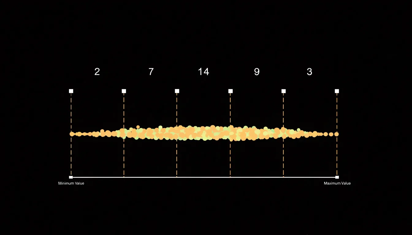
The shape emerging from these stacked intervals carries substantial information:
- Positive skew: A long tail stretching to the right tells you a handful of unusually large values pull the mean upward while most observations sit lower.
- Symmetry: A bell-like profile suggests the mean and median land near each other and that standard summary statistics are reasonably representative.
- Bimodality: Two distinct peaks often signal that two underlying populations have been mixed together, such as sales from two different regions pooled into one dataset.
- Modal interval: The tallest bar indicates where values cluster most densely, offering a quick read on central tendency before formal calculation.
Bin width matters considerably. Too few bins compress the data into a coarse block that hides structure; too many produce a spiky outline dominated by sampling noise. Trying several widths is a sound habit. Because the area of each bar corresponds to the proportion of observations, histograms also lend themselves to overlaying density curves or comparing subsets by transparency.
Density Plot
A density plot offers a smoothed representation of a distribution by transforming individual observations into a continuous curve describing the relative likelihood of values across a range. Rather than grouping data into discrete buckets, it estimates a probability density function directly from the sample using kernel density estimation (KDE). KDE places a small kernel function—commonly a Gaussian bell curve—at every data point. Each kernel contributes a localized bump of probability mass; the estimation sums these bumps and scales the result so the total area under the curve integrates to one.
While the kernel function determines the shape of each bump, a parameter called the bandwidth controls how wide each bump spreads. A small bandwidth yields a curve that tracks the data closely, revealing fine-grained features alongside random noise. A larger bandwidth produces a smoother, generalized curve emphasizing overall structure. Choosing an appropriate bandwidth balances sensitivity to local detail against the clarity of the broader shape.
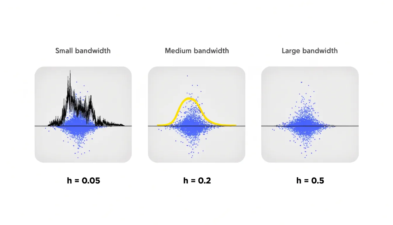
Because density plots avoid rigid bin boundaries, they sidestep a common weakness of histograms, where the visual impression can shift depending on where bin edges fall. The continuous curve makes it easy to spot skewness, multimodality, and tail weight at a glance. This makes density plots especially useful for comparing several distributions on shared axes, since overlapping curves communicate differences in location, spread, and shape directly without the visual clutter of overlapping bars.
Box Plot
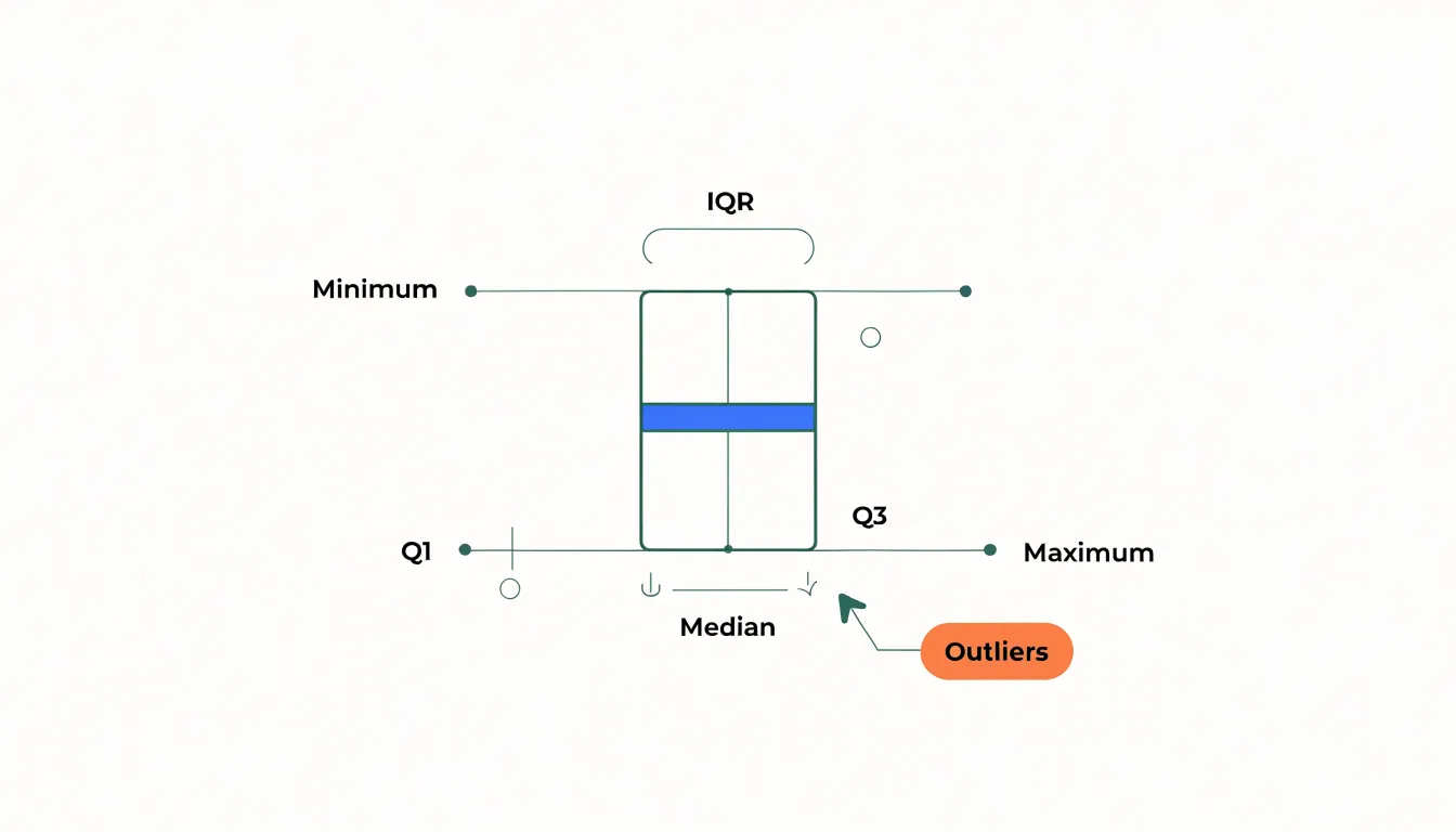
A box plot condenses a dataset into a five-number summary: the minimum, first quartile, median, third quartile, and maximum. The central box spans the interquartile range (IQR) from the first to the third quartile, containing the middle half of all observations. A line inside the box marks the median, while whiskers extend outward toward the minimum and maximum values to show overall spread. Together, these five numbers show where a distribution is centered, how widely it disperses, and whether it leans toward one side.
The real power of a box plot emerges when placing several side by side along a shared axis. Medians line up for direct comparison, and differences in spread or skew become immediately visible. Analysts can quickly see which category produces higher values, which is more variable, and which is tightly clustered—making box plots routine in experimentation, quality control, and survey analysis.
Outlier identification is another core strength. Points falling far beyond the whiskers are plotted individually, flagging unusually high or low observations that might signal data entry errors, rare events, or anomalies worth investigating. Because the summary relies on quartiles, a handful of extreme values cannot distort the overall shape. Box plots also pair well with strip plots or jittered points, showing both the statistical summary and the underlying observations.
Violin Plot
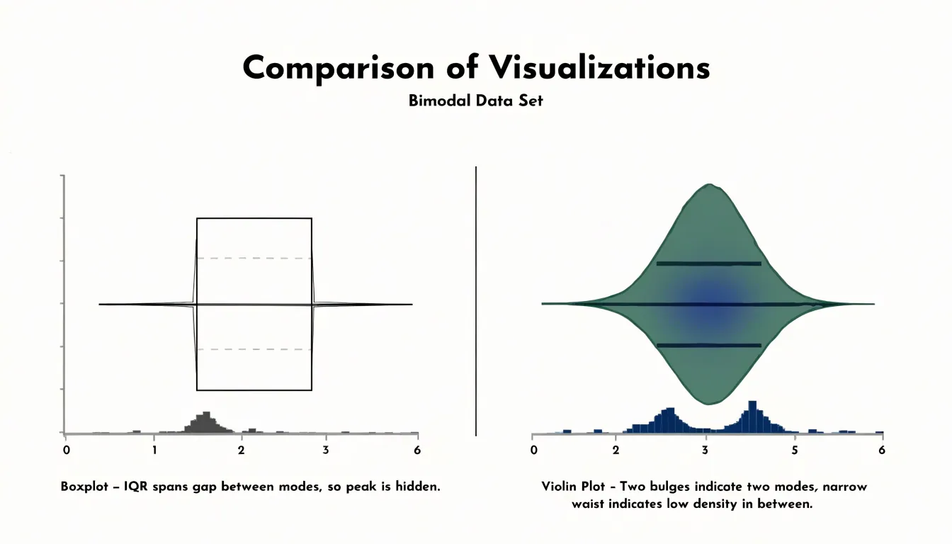
A violin plot combines a kernel density estimate with the summary metrics of a box plot. The outer outline draws the density curve symmetrically on both sides of a central axis, creating a violin-like silhouette that makes the widest, densest regions easy to compare visually. Inside that outline sit markers for the median and the interquartile range, showing the full shape of the distribution alongside compact statistics for its center and spread.
This combination excels with multimodal data. A box plot alone can hide values clustering around two distinct peaks because the interquartile range simply spans the gap between them. The violin’s density outline narrows in the middle and swells at each peak, showing a bimodal distribution as two bulges separated by a waist. Anyone scanning a row of violins can spot these waists quickly and recognize that a single summary like the mean would be misleading. The density estimate also reveals skew, long tails, and sharp spikes that a five-number summary smooths away, while the internal median and quartile markers provide precise reference points for comparing groups side by side.
Strip Plot
A strip plot places one marker for each observation along a single value axis, preserving the full raw dataset without aggregation, binning, or summarization. When observations are few enough that markers remain distinguishable, this one-point-per-record approach gives readers complete transparency. Viewers can count records, spot exact values, and see where density naturally clusters.
Without adjustment, points sharing identical or similar values fall on top of one another. Adding a small random offset along a cross axis—a technique called jittering—separates coincident markers to reveal how many records sit at each position. Jittering introduces slight artificial displacement on the cross axis while keeping the measured value axis accurate. An unjittered strip plot stacks points directly on their true values and works best when data contain limited distinct values.
Strip plots are most effective with smaller datasets, often up to a few dozen observations, where individual markers remain visible, or with discrete measurements where stacking conveys frequency. For larger samples, points merge into an opaque band, requiring designers to pair the strip plot with a summary overlay (like a box plot) or shift to a denser representation.
Swarm Plot
A swarm plot (or beeswarm plot) also plots individual data points along a categorical axis, but instead of random jittering, it uses an algorithm to offset points horizontally so no two markers overlap. The algorithm typically sorts points by value and iteratively places each one at the smallest available cross-axis offset that avoids collision with previously placed points.
This keeps every point at its exact position on the numerical axis while creating a symmetrical, swarm-like silhouette that reveals the density and shape of the distribution. Like strip plots, swarm plots preserve individual observations, making it easy to identify clusters, gaps, and outliers across categories. However, because points cannot overlap, large datasets cause the horizontal spread to grow too wide, making swarm plots best suited for small to moderate sample sizes.
Ridge Plot
A ridge plot, sometimes called a joyplot, arranges several density curves as a vertical stack, each shifted slightly upward and partially overlapping the curve behind it like receding ridgelines. This layout lets you compare many distributions at once along a shared horizontal axis.
Suppose you track household incomes across a decade, one ridge per year. A gradual movement of the peak toward higher values appears as a slow drift down the stack. A widening base signals growing inequality, and a new bump in the low-income region points to a subgroup entering the population. The same logic applies to categories like product ratings by region, test scores by school, or reaction times by experimental condition. The stacking order itself becomes a meaningful dimension—often time or rank—reading like a topographic profile of change.
Partial overlap makes this compact view possible: fully separated curves force the reader to jump between distant panels, while complete overlap on a single baseline creates a tangled mess. Designers typically keep the overlap moderate and use light fill colors with crisp outlines so each ridge remains traceable, anchoring the comparison with row labels on the left edge.
Cumulative Distribution Plot
A cumulative distribution plot shifts focus from bin frequencies to the running total of data across a range. Dividing this running total by the sample size yields the empirical cumulative distribution function (ECDF): a step function increasing from 0 to 1, where each vertical step corresponds to an observed value. The curve’s height at any x-value represents the proportion of observations less than or equal to that value.
This makes percentiles and thresholds immediately readable. The median is the x-value where the curve crosses 0.5, and the 90th percentile is where it crosses 0.9. In a dataset of customer ages, an ECDF lets you read directly that 75% of customers are younger than 42.
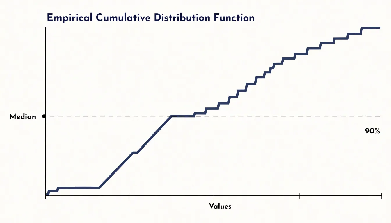
Unlike histograms or density plots, the ECDF requires no binning or bandwidth tuning, displaying all data points without arbitrary grouping or smoothing. It handles skewed data and outliers gracefully, as heavy tails or gaps appear clearly in the slope of the steps. Plotting multiple ECDFs on the same axes works exceptionally well for comparing groups—such as before and after an intervention—making it easy to see exactly where and by how much the distributions diverge.
Dot Plot
A dot plot (specifically a Wilkinson dot plot) places a circular marker for each observation above its value on a horizontal axis, stacking repeated values vertically so column height encodes frequency. For small datasets—particularly discrete counts like household members, weekly purchases, or survey responses on a five-point scale—this visual tally shows distribution shape without intermediate calculation.
Because every observation remains visible as a countable dot, nothing is hidden: a single outlier appears as a lone dot, and repeated values form clear stacks. That fidelity matters when samples are too small for histograms (which look blocky) or density curves (which imply unsupported smoothness). Discrete values like 0, 1, 2, or 3 sit at labeled positions with empty space between them, matching the data’s true nature and requiring no statistical background to interpret.
Q-Q Plot
A Q-Q (quantile-quantile) plot provides a graphical method for assessing whether a dataset follows a theoretical distribution, most commonly the normal distribution. To construct it, you sort the observed sample values to find their empirical quantiles and plot them against the corresponding theoretical quantiles from the reference distribution on a scatterplot. If the data follow the theoretical distribution, the points fall closely along a straight diagonal line.
The plot’s value lies in reading departures from that diagonal:
- S-shaped curve: Points curving upward at the right end and downward at the left indicate the sample has heavier tails (more extreme values) than the theoretical model predicts.
- Flattened ends: Points bending in the opposite direction suggest lighter tails and a more bounded distribution.
- Isolated departures: Individual points sitting far off the line at either end flag potential outliers.
Q-Q plots complement numeric normality tests by showing where and how data deviate across the entire range, rather than reducing the assessment to a single pass-or-fail statistic.
Heatmap
A two-dimensional heatmap extends the histogram into bivariate space. Instead of binning along a single axis, it divides the plotting plane into a grid, counts how many data points fall inside each cell, and maps that count to color intensity. Dense regions glow brightly while sparse regions fade, creating a compact picture of a joint probability distribution.
This approach solves the overplotting problem in scatter plots, where thousands of overlapping points collapse into an unreadable cloud. Binning the plane and mapping counts to a sequential color palette recovers the underlying structure: clusters appear as saturated patches, ridges trace the relationship between the two variables, and isolated outliers show up as faint single cells at the grid’s edges. As with one-dimensional histograms, large grid cells emphasize broad trends while small cells preserve fine detail at the cost of visual noise; some tools also apply smoothing to blend neighboring cells into a continuous 2D density surface.
Choosing a Chart by Sample Size and Outliers
Sample size, extreme values, and audience familiarity should guide your chart selection:
- Small samples (up to a few dozen): Every point carries weight. Use a dot plot, strip plot, or swarm plot to show individual values without smoothing away detail.
- Medium samples (dozens to low hundreds): Histograms and box plots efficiently summarize spread and central tendency.
- Large samples (thousands+): Density plots, violin plots, and 2D heatmaps handle high volume gracefully, whereas unbinned strip or scatter plots collapse into indistinguishable smudges without transparency or aggregation.
When outliers are the main story, box plots explicitly flag points beyond the whiskers, and strip plots or Q-Q plots keep every extreme observation visible. Conversely, wide histogram bins can swallow outliers into a bar, and kernel density smoothing can trim their influence. If outliers are mere noise, robust summaries like the median and IQR keep the main pattern readable, while logarithmic axes can help manage extreme positive skew.
Finally, match the encoding to your audience. Technical readers appreciate box plots, violin plots, and ECDFs for their statistical precision. General audiences often respond better to simple histograms, dot plots, or annotated density curves. Presentation slides reward clean, sparse summaries, while interactive dashboards can support layered views with tooltips and filters.
Avoiding Common Pitfalls
Choices around axis scales and binning heavily influence how readers interpret a distribution:
- Truncated axes: Starting a frequency bar’s axis above zero exaggerates differences between bins. While narrowing the value axis range is sometimes appropriate for dot plots or box plots to focus on a tight cluster, cutting off the tails of a distribution hides outliers. Always inspect the full data range before setting axis limits, and clearly cue any shifted baselines.
- Unchecked bin widths: In histograms, too few bins cause over-smoothing that hides distinct modes or gaps, while too many create a noisy profile where random fluctuations look like structure. Test several widths to find a stable shape, using Sturges’ rule or the Freedman–Diaconis rule (especially for skewed data) as starting points.
- Mismatched scales and bins: When comparing histograms or density curves across groups, enforce identical axis limits, bin widths, and bin origins (anchor points), as shifting where bins start can shift apparent peaks. Watch for empty bins that suggest false gaps in sparse data.
- Unlabeled log scales: A logarithmic axis compresses large values and can make right-skewed data look symmetric. Always label logarithmic transformations explicitly on the axis.
Chart Selection Overview
You can treat chart selection as a lookup matrix pairing your analytical objective with the constraints of your data:
- Inspect the shape of a single variable: Use a histogram or density plot for moderate-to-large samples, or a dot plot or strip plot for small samples where preserving raw observations matters.
- Compare distributions across categories: Use side-by-side box plots or violin plots for a compact summary of medians, spread, and multimodality; use a swarm plot for smaller groups; or use a ridge plot when comparing across many ordered categories or time steps.
- Detect outliers and inspect tails: Use a box plot to flag extremes via IQR rules, or a Q-Q plot to evaluate tail behavior against a theoretical reference like the normal distribution.
- Evaluate cumulative thresholds and percentiles: Use an ECDF to read exact proportions below any value without binning distortions.
- Explore joint distributions of two variables: Use a 2D heatmap (or a scatter plot with marginal histograms) to reveal bivariate clusters and avoid overplotting.
Frequently Asked Questions
What is the difference between a histogram and a density plot?
A histogram breaks a continuous variable into adjacent bins and counts observations per bin, while a density plot uses kernel density estimation to create a smoothed continuous curve. Density plots avoid rigid bin boundaries, so the visual impression does not depend on where bin edges fall.
What does a long right tail in a histogram mean?
A long right tail indicates positive skew: a handful of unusually large values pull the mean upward while most observations sit lower.
When should I use a violin plot instead of a box plot?
A violin plot combines a kernel density estimate with box plot summary metrics and excels with multimodal data. A box plot alone can hide values clustering around two distinct peaks because the interquartile range simply spans the gap between them.
What sample size works best for a strip plot or swarm plot?
Strip plots are most effective with smaller datasets, often up to a few dozen observations, or with discrete measurements where stacking conveys frequency. Swarm plots are best suited for small to moderate sample sizes because large datasets cause the horizontal spread to grow too wide.
How do I read percentiles from a cumulative distribution plot?
On an ECDF, the curve’s height at any x-value represents the proportion of observations less than or equal to that value. The median is where the curve crosses 0.5, and the 90th percentile is where it crosses 0.9.
What should I watch out for when setting axis limits or bin widths?
Starting a frequency bar’s axis above zero exaggerates differences between bins, and cutting off distribution tails hides outliers; inspect the full data range before setting axis limits and clearly cue any shifted baselines. For histograms, too few bins hide structure while too many produce a noisy profile, so test several widths.
Tony Astor
Tony writes about data visualization and the tools people use to build charts and dashboards. More about Data Illustrator