How to Handle Outliers in Charts
 By Tony Astor ·
How to Handle Outliers in Charts
Handle outliers in charts by detecting them first—scatter plots expose them as isolated points, box plots flag values beyond 1.5×IQR—then addressing them: adjust scales (log, broken axis), trim or Winsorize extremes, or label anomalies with their cause. Use median instead of mean for skewed data, and always document any transformation.
Table of Contents
Scatter Plots
A scatter plot places every observation on a two-dimensional plane, with one variable on each axis, so that each individual data point appears as a separate mark. This one-to-one mapping between records and visible marks gives the chart its diagnostic strength. When unusual values exist, they often reveal themselves as points sitting far from the main cloud, isolated at an extreme of one axis, or forming small clusters that drift away from the overall trend. Because nothing is aggregated or summarised into a single line or bar, these anomalies stay visible instead of being averaged away.
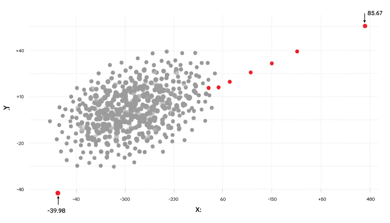
The real value of the scatter plot emerges in exploring relationships between variables. A dense central mass of points usually indicates the typical joint behaviour of two measures, while any point positioned well outside that mass signals an unusual combination, such as a high value on one variable paired with a low value on the other. Plotting individual data points also exposes distinct grouping patterns: a subset of records may form a tight secondary cluster offset from the primary cloud, suggesting a subpopulation with different behaviour, a data entry problem, or a genuine divergence worth investigating.
Readability matters for spotting these patterns. Clear axis scales, sensible ranges, and light gridlines help viewers judge distance and position accurately. Overplotting can obscure isolated points when many observations share similar coordinates, so adjusting marker transparency, reducing marker size, or using jitter can help separate overlapping marks and keep lone outliers visible. A brief text note or annotation near a suspicious point can direct the reader’s attention to the discovery.
In practice, a scatter plot works best as an early exploratory step: it shows where outliers sit, how far they depart from the main pattern, and whether unusual values appear alone or in coherent groups, providing concrete evidence for deciding on further investigation or treatment.
Box Plots
Box plots offer a compact way to surface extreme values without inspecting every individual data point. The method begins by ordering the dataset and dividing it into quartiles. The first quartile (Q1) marks the point below which 25 percent of observations fall, the second quartile is the median, and the third quartile (Q3) marks the 75 percent boundary. The distance between Q1 and Q3 is the interquartile range, or IQR, which captures the spread of the middle half of the data and is far less sensitive to extreme observations than the full range.
The IQR then serves as the foundation for whisker thresholds. A common convention places the lower whisker at Q1 minus 1.5 times the IQR and the upper whisker at Q3 plus 1.5 times the IQR. Any point beyond those boundaries is plotted individually as an outlier, giving the reader an immediate visual cue that a value sits unusually far from the central mass of the distribution. A more conservative threshold of 3.0 times the IQR flags only far-out values, which is useful when mild departures are expected and would otherwise clutter the chart.
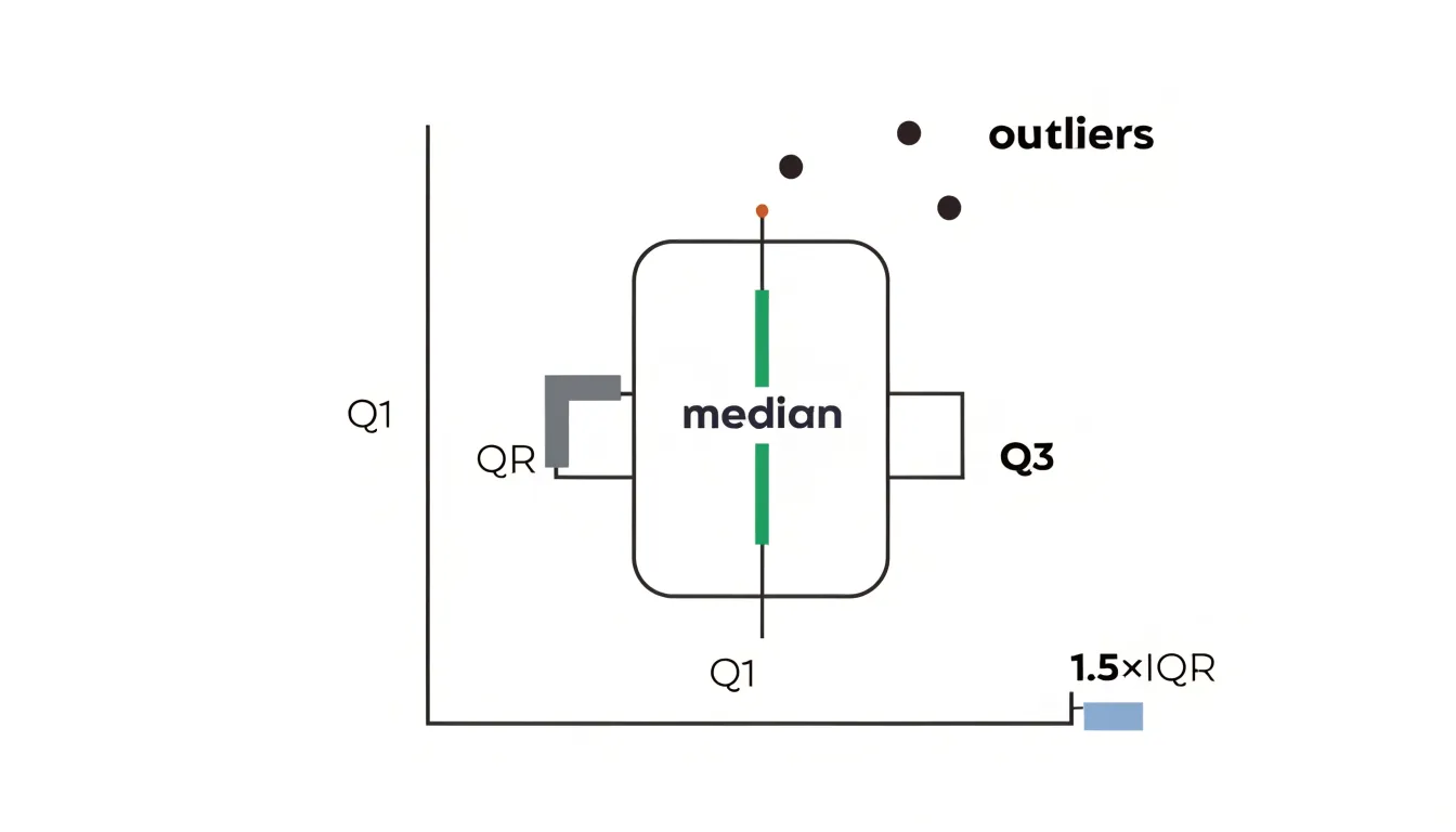
The practical benefit is that the rule is objective and repeatable. Rather than relying on personal judgment about what looks unusual, the thresholds derive from the data’s own spread, so the highlighted extremes reflect statistically significant departures from the typical range. This makes box plots well suited to comparing several groups side by side, since each box and its whiskers can be read against the others at a glance.
When building a box plot, document the multiplier you used and check whether hardware limits, known data entry errors, or genuine rare events explain the flagged points. Note also that the whisker rule assumes a roughly unimodal distribution, so heavily skewed data may produce many flagged values on the long tail, and the chart may benefit from a companion view or a note explaining the pattern.
Adjusting Chart Scales
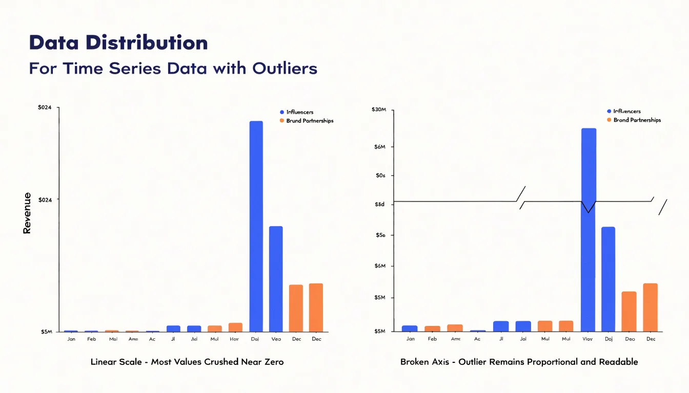
Adjusting chart scales is one of the most direct techniques for managing skewed axis layouts while preserving the context readers need. When a single high-magnitude outlier forces the axis to stretch toward an extreme value, the rest of the data set collapses into a narrow band near the origin, making genuine variation invisible. A common approach is to set an axis range that deliberately excludes the outlier’s full extent while flagging that exclusion clearly, for example with a broken axis marker or an annotation at the chart edge. Broken axes let you skip a stretch of empty scale between the main data cluster and the distant value, keeping the outlier visible as a distinct mark without sacrificing resolution in the densely populated region. Another technique is rescaling to a logarithmic axis, which compresses the distance between orders of magnitude so that both small and large values remain legible on the same plot. Log scales suit ratio-driven data such as growth rates or counts spanning several powers of ten, though they require explicit labeling so readers do not misread spacing as linear. For charts where the outlier is a known data error or an irrelevant extreme, capping the axis at a percentile-based maximum and noting the cap keeps the majority of the distribution readable. Whichever method you choose, the guiding principle is transparency: every recalibration should be visible in the axis labels, tick marks, or a short caption note. An unlabeled truncated axis can mislead as surely as an unreadable compressed one. Combining a narrowed range with a secondary inset chart for the outlier gives readers both the fine-grained view of the main data and the full picture of the extreme value. The goal is a scale that lets the primary pattern speak while the outlier remains acknowledged rather than erased.
Logarithmic Scales
Logarithmic scales offer a practical way to bring wide-ranging values onto a chart without letting a handful of large numbers dominate the entire visual. When data spans several orders of magnitude, a standard linear axis stretches itself to accommodate the highest value, and the smaller values collapse near the baseline where they become nearly indistinguishable. A log transformation changes this by plotting values according to their exponent rather than their raw magnitude. Each equal distance along the axis represents a constant multiplicative factor, whether tenfold, a hundredfold, or more, depending on the base chosen. This compression keeps both the very large and the very small values visible on the same canvas, so readers can trace patterns across the full range instead of squinting at a flat line near zero.
Exponential growth patterns benefit especially from this treatment. A series that doubles repeatedly appears as a gentle curve on a linear axis, flattening toward the left and shooting upward toward the right, which hides the consistency of the underlying growth rate. Plotted on a logarithmic scale, that same series becomes a straight line, making the steady proportional increase immediately apparent. Analysts use this property to test whether growth is truly exponential: if the logged values form a roughly straight trend, the rate of change is constant in relative terms.
Log scales also help when extreme values create massive jumps that would otherwise distort a chart’s proportions. A single outlier reaching into the millions can render every other data point invisible on a linear axis, while a logarithmic view pulls that outlier into a position where the rest of the distribution remains readable. The trade-off is interpretive: equal vertical distances no longer represent equal absolute amounts, so labels and annotations should state clearly that the axis is logarithmic. Readers unfamiliar with log scales sometimes misjudge the magnitude of differences, particularly in the lower regions of the chart, so pairing the transformed view with a clear note or a secondary linear reference helps maintain honest communication of the data.
Break Scales
When a chart must display both a dramatic spike and subtle baseline variations at the same time, a single continuous axis often forces a compromise that serves neither. A break in the scale offers a way out. The idea is to compress or skip a range of values on an axis so that the space between the ordinary readings and the extreme spike is visually reduced. The result is a chart in which the spike remains visible and proportionate without flattening the small movements that carry much of the story.
Implementing a break begins with identifying the gap in the data. If most values sit between 10 and 40 while a handful reach 900, the empty band between roughly 50 and 850 is a candidate for compression. The axis is then drawn with two segments, each with its own range, joined by a visual marker. Common markers include a pair of short parallel slashes across the axis line, a zigzag, or a small gap in the plotting area itself. The marker signals to the reader that the scale is not continuous and that distances across the break should not be compared directly.
Safety comes from consistency and clear labeling. Every series on the chart should share the same break points, so bars or lines remain comparable to one another. Tick labels on both sides of the break should stay visible, and the marker should be placed where it cannot be mistaken for a data point. Annotating the break with a brief note, or mentioning it in the chart title or caption, reinforces the message. Used this way, a scale break keeps the spike honest while preserving the detail of the baseline, and readers retain a trustworthy sense of both.
Trimming Extreme Values
Trimming extreme values is one of the most practical ways to clean up a chart without losing the story the data is trying to tell. A single fluke measurement, such as a sensor misfire, a data entry slip, or an unusually large one-off transaction, can stretch a chart’s axis so far that every meaningful movement in the rest of the series flattens into a straight line. Trimming addresses this by removing or limiting those non-representative anomalies so the genuine trend becomes visible again. The key principle is that the values you adjust should be ones you can reasonably argue do not belong to the phenomenon you are charting, rather than merely values that look inconvenient.
Two standard techniques do most of the work. Truncation, sometimes called trimming in the strict sense, simply removes the extreme observations from the dataset before plotting. You define a threshold, such as the top and bottom one percent of values, and drop anything beyond it. This is straightforward and transparent, though it does discard information, and the chart then describes only the retained portion of the data. Winsorizing takes a gentler approach: instead of deleting extremes, it caps them at a chosen percentile, so a value in the top one percent is replaced with the value at the ninety-ninth percentile. The observation stays in the dataset, preserves its ordering, and no longer dominates the scale. Winsorizing is often preferable when the extremes are real but unrepresentative, since it keeps every record while limiting each one’s influence on the chart’s shape.
Whichever method you choose, document the threshold and the rule you applied, ideally in a note beneath the chart. Readers should know that the axis reflects adjusted data and where the cutoffs sit. Applied carefully, trimming and winsorizing keep the underlying story intact while freeing the visual from the distorting pull of a handful of anomalies.
Comparing Median Averages
When a dataset contains extreme values, the arithmetic mean can be misleading. A single very high or very low observation pulls the mean toward that extreme, shifting the apparent center of the data away from where most values actually lie. This sensitivity makes the mean a fragile measure of central tendency in the presence of outliers. The median, by contrast, depends only on the rank order of values. It identifies the middle value when data are sorted, so any number of extreme observations at either end affect it only by changing the position of the middle, not by pulling it toward the extremes. For example, in a set of house prices where most homes are around $300,000 but one sells for $30 million, the mean will be inflated far above what a typical home costs, while the median remains close to the typical value. The mode, the most frequently occurring value, offers another stable perspective, particularly for categorical or discrete data. It is entirely unaffected by the magnitude of outliers, since it depends only on frequency. In distributions with a clear peak, the mode can reveal the most common value even when the mean and median are distorted. Together, median and mode provide a more robust summary of central tendency when data contain severe high or low extremes. They help analysts and readers avoid drawing false conclusions from a mean that has been skewed by a few unusual cases. By comparing these stable metrics alongside the mean, one can assess the influence of outliers and choose the measure that best represents the typical observation. This approach is especially important in fields like income analysis, real estate, and performance reporting, where extreme values are common and can distort summary statistics.
Labeling Chart Anomaly Points
Labeling chart anomaly points transforms a puzzling spike into a readable story for stakeholders. When a line chart suddenly jumps or a bar towers above its neighbors, viewers naturally ask what happened. A callout annotation placed directly beside the point answers that question at the moment it arises, pairing a short descriptive label with the value and the reason behind it. For example, a sales dashboard showing a sharp increase in March might carry a callout reading “March spike: spring promotion launched, +42% versus February.” The annotation sits on the chart itself, so the explanation travels with the visual wherever it is shared, pasted into a slide deck, or reviewed in a meeting.
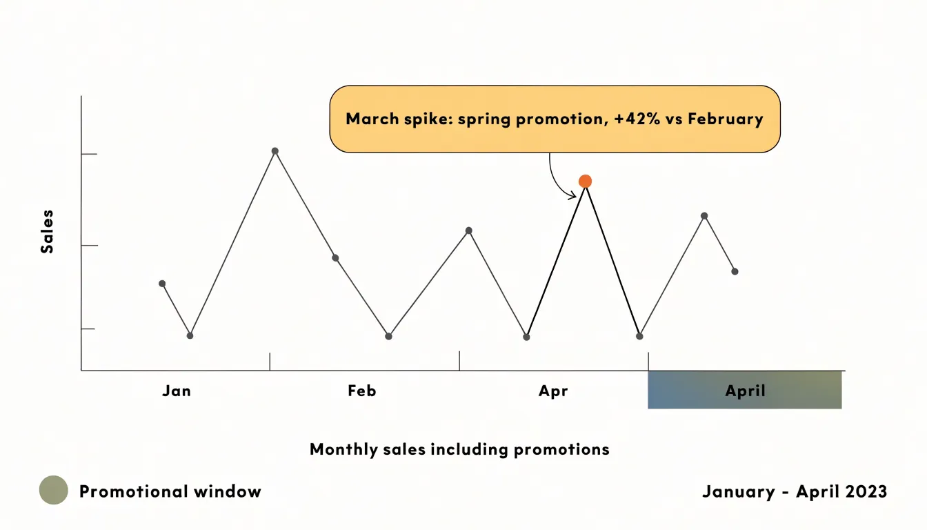
Effective callouts combine three elements: a clear label naming the event, the measured value or percentage change, and a brief note on the cause. The label should use plain language that a non-analyst can absorb in seconds. Positioning matters as well; the annotation should point precisely at the data point without obscuring neighboring values or gridlines. A thin leader line connecting the text box to the spike keeps the association unambiguous.
Descriptive text also plays a role beyond the chart frame. A short caption beneath the visual, or a sentence in the accompanying narrative, can explain why the anomaly is valid and what it means for the business. This is especially important when the spike reflects a real, business-impacting event such as a product launch, a seasonal surge, or a one-time marketing push. By naming these causes explicitly, the chart communicates that the outlier is understood and intentional, which builds confidence in the analysis.
Well-labeled anomalies also reduce follow-up questions. Stakeholders can interpret the chart on their own, and reviewers spend less time chasing explanations. The overall goal is to make every unexpected result self-explanatory, so the chart supports decisions rather than prompting confusion.
Spotting Data Entry Errors
Data entry errors are among the most common sources of misleading charts, and they often originate from simple human mistakes. A single mistyped digit can transform a revenue figure of 5,000 into 50,000, and a misplaced decimal point can turn a modest 12.5 percent growth rate into 125 percent. When these mistakes flow directly into a visualization, the resulting chart may show dramatic spikes, implausible dips, or distorted trends that draw attention away from the real story in the data. Catching these errors before plotting is therefore a core step in preparing any dataset for chart generation.
A practical pre-cleansing routine starts with scanning numeric columns for values that fall outside plausible ranges. A quarterly sales figure that exceeds the annual total, a customer age recorded as 250, or a temperature reading of 999 degrees all point to fat-finger mistakes or placeholder entries that were never replaced. Setting sensible minimum and maximum thresholds for each field makes these outliers easy to flag for review.
Misplaced decimals deserve particular attention because they can produce values that look superficially reasonable. An invoice amount entered as 45.00 instead of 4,500, or a measurement recorded as 0.75 when the instrument reports 75, shifts the scale of an entire axis without obviously violating any range rule. Comparing each value against the typical magnitude of its column, or checking decimal place counts, helps surface these inconsistencies.
Formatting glitches form a third category. Numbers stored as text, inconsistent units, stray currency symbols, or dates entered in mixed formats can all cause plotting tools to misinterpret values or drop records silently. Standardizing formats and converting text fields to numeric types during cleansing prevents these issues from reaching the chart stage.
Building a short review checklist and running it on every raw dataset before plotting keeps these errors from distorting your visuals and the decisions they inform.
Filtering Customer Ratings
Customer rating charts are among the most visible signals of product health, which makes them a frequent target for manipulation. Spam reviews and coordinated rating campaigns can push a product’s average score sharply upward or downward within a short window, and when those spikes appear in a feedback chart they distort the picture of what real customers actually think. Filtering these entries begins with recognizing the patterns that distinguish them from organic activity. Bot-generated reviews often arrive in tight clusters, share near-identical timestamps, use repetitive or template-like language, and come from accounts with little or no purchase history. Fraudulent rating spikes frequently show a sudden concentration of five-star or one-star scores with no corresponding change in sales volume, support tickets, or page engagement.
Once suspicious entries are identified, the next step is deciding how to handle them in the chart itself. One approach is to remove flagged reviews from the dataset entirely before calculating averages, then annotate the chart to note that a filtering step was applied. Another is to display the raw and filtered averages side by side so viewers can see how much the outliers influenced the original figure. Segmenting ratings by verified versus unverified purchases offers a further layer of clarity, since verified reviews tend to reflect genuine customer experience more reliably.
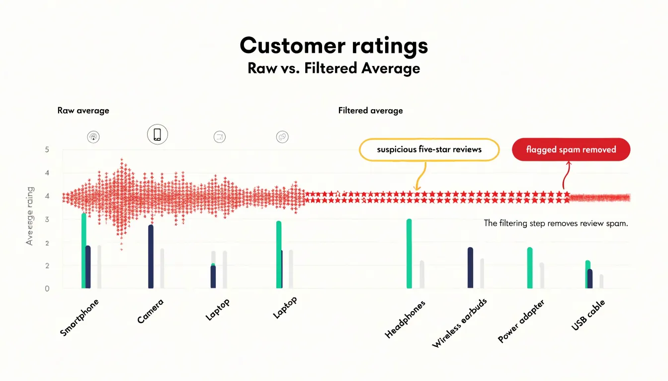
The goal throughout is an honest representation of customer sentiment. Filtering should be documented and repeatable, using consistent criteria so that the chart remains trustworthy over time. Analysts should also monitor filtered-out volume as a metric in its own right, because a rising share of spam activity may indicate a broader integrity problem worth addressing with the platform or review provider. Handled this way, rating charts become a dependable window into how customers truly feel about a product.
Keeping Original Records
Keeping original records means storing the unaltered raw data exactly as it was collected, before any cleaning, transformation, or filtering takes place. This unedited baseline dataset serves as a reference point for audits, compliance checks, and verification of any charts or analyses derived from it. When you apply transformations to handle outliers—such as removing extreme values, capping them, or applying statistical corrections—you create a modified version of the data. Without the original records, it becomes impossible to trace back to the source and confirm that the transformations were applied correctly and consistently. For compliance purposes, many industries and regulatory frameworks require organizations to maintain raw data for a specified period. An unedited baseline ensures that you can demonstrate the provenance of your chart data, showing exactly what was changed and why. This is particularly important when outliers are excluded: auditors may want to see the full dataset, including the outliers, to assess whether their removal was justified. Verification also benefits from having the original records. If a chart is questioned, you can reproduce the entire pipeline from raw data to final visualization, confirming that no errors were introduced. Storing raw data separately from transformed data also prevents accidental overwrites or loss. A common practice is to keep raw data in a read-only format or in a dedicated archive, with clear documentation of any processing steps. This way, the original records remain intact and accessible whenever needed. Ultimately, maintaining an unedited baseline supports transparency and trust in the charts you produce, especially when outliers have been handled in ways that materially affect the results.
Final Chart Reviews
A final chart review is your last opportunity to catch issues that automated checks might miss. Begin by stepping back and assessing visual balance. Does the chart feel cluttered or sparse? Are elements like gridlines, legends, and annotations competing for attention? Adjust the layout so the data remains the focal point. Check that colors are used consistently and that contrast is sufficient for readability, especially for viewers with color vision deficiencies. Next, verify data integrity. Confirm that all outliers have been handled according to your chosen method and that the chart accurately reflects the underlying data. Look for any accidental distortions, such as truncated axes or inconsistent scales, that could mislead. Ensure that totals and percentages add up correctly and that any transformations (e.g., logarithmic scales) are clearly indicated. Finally, scrutinize explanatory labels. Titles should be clear and descriptive, subtitles can provide context, and axis labels must include units. Annotations should highlight key insights without overwhelming the viewer. Check that all text is legible at the intended display size and that abbreviations are defined. At this stage, it’s also wise to consider the audience: will they understand the chart without additional explanation? If not, add a brief note or adjust the design. Performing this sanity check routinely before publishing reports ensures that your graphics communicate effectively and instill confidence in your findings. A clean, well-labeled chart not only conveys information but also reflects the care taken in the analysis, enhancing your credibility and the impact of your report.
Frequently Asked Questions
How can a scatter plot help identify outliers?
A scatter plot places every observation as a separate visible mark, so unusual values often show up as points far from the main cloud, isolated at an extreme of one axis, or in small clusters drifting away from the trend. Because the data are not aggregated into a single line or bar, these anomalies stay visible.
What is the 1.5 IQR rule for outliers in a box plot?
A common convention places the lower whisker at Q1 minus 1.5 times the IQR and the upper whisker at Q3 plus 1.5 times the IQR, with points beyond those boundaries plotted individually as outliers. A more conservative threshold of 3.0 times the IQR flags only far-out values.
When should I use a logarithmic scale for data with outliers?
A logarithmic scale is useful when data spans several orders of magnitude or when extreme values would otherwise make smaller values nearly indistinguishable. It plots values by exponent so equal distances represent a constant multiplicative factor, but labels and annotations should clearly state that the axis is logarithmic.
How do you add a break to a chart scale correctly?
Identify the gap in the data, then draw the axis in two segments with a visual marker such as parallel slashes, a zigzag, or a gap in the plotting area. Every series should share the same break points, tick labels on both sides should stay visible, and the break should be annotated or mentioned in the title or caption.
What is the difference between trimming and winsorizing extreme values?
Trimming, or truncation, removes extreme observations beyond a chosen threshold from the dataset before plotting. Winsorizing caps extremes at a chosen percentile, so the observation stays in the dataset but no longer dominates the scale; either way, document the threshold and rule applied.
Why should I keep original records when handling outliers?
Keeping original records means storing the unaltered raw data before any cleaning, transformation, or filtering, providing a baseline for audits, compliance checks, and verification. Storing raw data separately, such as in a read-only format or dedicated archive with documentation, helps prevent accidental overwrites or loss.
Tony Astor
Tony writes about data visualization and the tools people use to build charts and dashboards. More about Data Illustrator