How to Choose the Right Chart for Your Data
 By Tony Astor ·

How to Choose the Right Chart for Your Data
Choose a chart by the question being answered: bar charts compare categories, line graphs show change over time, pie and ring charts show part-to-whole, histograms and box plots reveal distribution, scatter plots show relationships between two variables, choropleth maps display regional patterns, and Sankey, waterfall, and tree map charts trace flows, cumulative change, and hierarchy.
Table of Contents
Bar Charts
Bar charts are the workhorse for comparing values across categories, and the orientation you choose shapes how easily readers can make those comparisons. Vertical bars suit a modest number of categories with short labels, letting the eye scan heights against a common baseline. Horizontal bars become the better choice when category names are long, when there are many categories, or when labels would otherwise rotate or truncate along the x-axis. Horizontal layouts also give the eye a natural left-to-right reading path that matches how many audiences scan text, which helps longer labels stay legible without crowding.
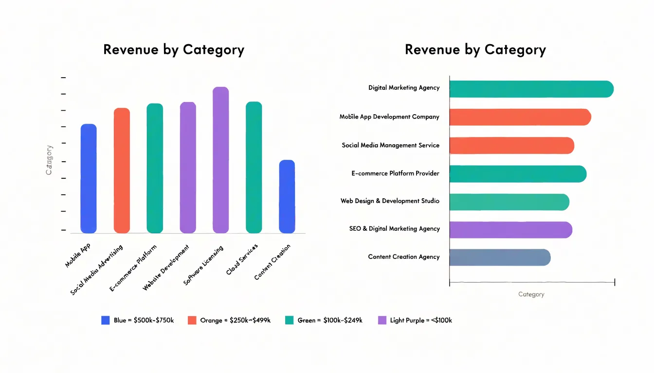
Ordering categories is where much of a bar chart’s communicative power lives. Alphabetical order works for lookup tasks, but sorting bars by value, either descending or ascending, turns the chart into a ranked story and makes the largest and smallest values immediately visible. When categories have an inherent sequence, such as age brackets or satisfaction levels, preserve that natural order so the chart reflects the underlying scale rather than an arbitrary ranking.
Maintaining zero-baseline integrity is essential because bar length encodes magnitude. Truncating the axis exaggerates differences and can mislead readers about proportions. A bar chart should begin at zero so that a value twice as large appears twice as long. If the data range makes differences hard to see at full scale, consider alternatives such as a dot plot or a small-multiple layout rather than cutting the axis. Keep gridlines subtle, label values directly where useful, and use consistent bar widths to avoid visual distortion.
Line Graphs
Line graphs excel at showing how values evolve across a continuous time axis, making them the default choice whenever the story of your data is about movement, direction, or rate of change. The first decision is the time interval. Daily data can reveal sharp movements but often drowns the underlying pattern in noise, while monthly or quarterly aggregation smooths the line and clarifies direction. Match the interval to the decisions your audience makes: operational teams may need daily granularity, while executives reviewing annual performance are better served by quarterly or yearly points. Too many data points compress the horizontal axis and turn the line into a jagged thicket.
Multiple series add richness and risk. Limit the number of lines to what a reader can distinguish at a glance, typically four to six, and use color, line style, or direct end-of-line labels rather than a crowded legend. Consistent color assignments across charts help readers carry meaning from one figure to the next. When series have very different magnitudes, consider a secondary axis with clear labeling or split the chart into small multiples so no line is flattened into irrelevance.
Finally, decide whether the chart should emphasize long-term trends or short-term fluctuations. A trend line, moving average, or shaded confidence band can foreground the broader trajectory while still showing the raw data underneath. If short-term volatility is the point, keep the raw series prominent and annotate spikes with brief context. Label axes clearly, start the vertical axis at zero where honest comparison matters, and annotate significant events directly on the chart.
Pie and Ring Charts
Pie and ring charts are classic tools for showing how individual categories contribute to a total. Each slice’s angle is proportional to its share of the whole, making them intuitive for simple part-to-whole comparisons. However, their effectiveness drops sharply as the number of slices increases. Research and practical experience show that people struggle to compare angles and arc lengths accurately, especially when slices are similar in size. With more than five slices, the chart becomes cluttered, labels overlap, and the visual hierarchy collapses. In such cases, a bar chart or a stacked bar chart is often a better choice, as it allows for easier comparison of individual values.
Ring charts, also known as donut charts, address some of these limitations. By removing the center, they create space for a central label or key metric, such as a total or an average. This makes them ideal for dashboards where you want to combine a part-to-whole breakdown with a headline number. Donut charts also work well when you need to emphasize the overall composition rather than precise comparisons between slices, though the same five-slice rule of thumb applies.
To highlight a primary proportion metric, consider using a donut chart with a single slice pulled out or rendered in a contrasting color, or place the key percentage in the center. For pie charts, a common technique is to separate the most important slice slightly from the rest. Avoid using 3D effects or exploded slices for multiple categories, as these distort perception. When the goal is to focus on one dominant share, a simple two-slice pie or a donut with a large central figure can be powerful, provided the highlighted metric is clearly labeled.
Histograms and Box Plots
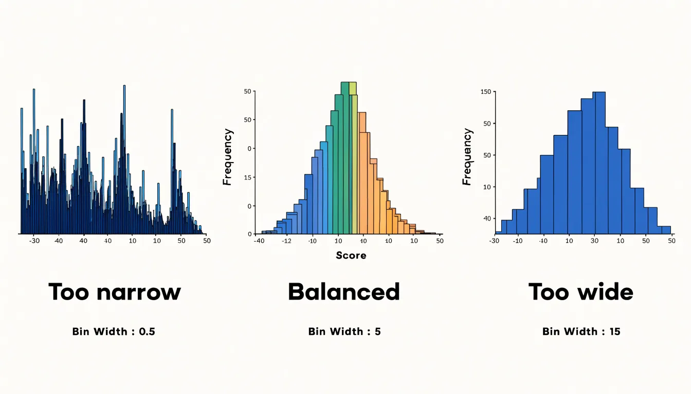
Histograms and box plots both answer questions about how a set of numbers is spread out, and each offers a distinct view of that spread. When building a histogram, the single most consequential decision is bin width. Too few bins compress real structure into a few coarse blocks, while too many bins scatter the data into a noisy comb of spikes that obscures the underlying shape. A useful starting point is to divide the range of values by the square root of the number of observations, which usually produces a readable number of bins for moderate datasets. For larger or more skewed datasets, a rule based on the interquartile range and the cube root of the sample size adapts better, because it widens bins when the data are tightly clustered. Whatever rule you apply, try two or three neighboring bin widths and compare the results; a genuine pattern persists across reasonable widths, whereas an artifact appears and disappears.
Box plots summarize spread through quartiles. The box spans the first quartile to the third quartile, so its height is the interquartile range, which contains the middle half of the observations and is resistant to extreme values. The line inside the box marks the median, and its position relative to the box edges reveals skew: a median pushed toward the lower quartile suggests a long upper tail, and vice versa. Whiskers typically extend to the most extreme values within 1.5 times the interquartile range from the box, and points beyond that threshold are plotted individually as outliers. Those points deserve a second look rather than automatic deletion, since they may signal data-entry errors, a separate population, or genuinely rare but important cases. Where a histogram shows the full shape of a distribution, a box plot condenses it into a compact, comparison-friendly summary, making the two methods effective companions.
Scatter Plots
Scatter plots are the go-to chart for exploring how two numeric variables relate to one another. Each point represents a single observation, positioned along a horizontal axis for one variable and a vertical axis for the other. The arrangement of those points reveals the shape of the relationship at a glance: whether values rise together, move in opposite directions, or show no discernible pattern at all. When reading a scatter plot, look for the overall direction of the cloud, the tightness of the clustering, and whether the pattern follows a straight line or curves. A tight diagonal band suggests a strong correlation, while a loose, formless cloud indicates the variables are largely independent.
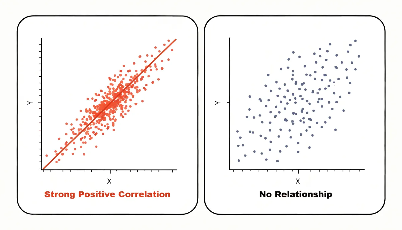
Dense datasets create a common problem called overplotting, where many observations land on the same or nearby coordinates and obscure one another. Transparency offers a simple fix: rendering points with partial opacity lets overlapping marks accumulate into darker areas, so you can see where observations concentrate. Jittering is another option, nudging points slightly off their exact positions to break up stacks and reveal density that would otherwise hide behind a single visible dot. Use jitter sparingly, since too much displacement can distort the true positions of your data.
Adding a trendline turns a scatter plot from a picture of individual observations into a summary of the statistical pattern. A linear fit draws a straight line through the cloud to show the average direction of the relationship, and an accompanying confidence band communicates how certain that estimate is. Curved or smoothed trendlines can capture nonlinear patterns that a straight line would miss. Trendlines are most useful when the underlying relationship is reasonably consistent; when the data splits into distinct clusters, consider coloring or faceting the points by group so each trendline reflects a coherent subset.
Choropleth Maps
Choropleth maps color geographic regions to represent data values, making them effective for showing regional patterns. To create accurate maps, normalize data by population or land area. Raw counts can mislead because larger regions may appear more significant simply due to size. For example, a map of total COVID-19 cases would highlight populous states, while a map of cases per capita reveals underlying risk. Similarly, population density (people per square kilometer) normalizes by land area and is useful for comparing settlement patterns. Choose a normalization that matches your analytical question: rates, ratios, or percentages are common.
When selecting color ramps, consider data type and purpose:
- Sequential ramps (light to dark) suit ordered data like income levels.
- Diverging ramps (two hues with a neutral middle) work for data with a meaningful midpoint, such as change in unemployment.
- Qualitative ramps (distinct hues) fit categorical data, though choropleths typically show quantitative data.
Beware of geographic size bias: large, sparsely populated regions dominate visually, while small, dense areas may be overlooked, distorting perception of the data’s distribution. To mitigate this, consider using cartograms that scale regions by population or other variables, or pair the map with a complementary chart like a bar graph. Additionally, choose appropriate class breaks (e.g., quantiles, equal intervals, natural breaks) to avoid misleading patterns, and always include a clear legend and data source.
Grouped and Stacked Bar Charts
Grouped and stacked bar charts both let you compare multiple metrics at once, and the choice between them hinges on what question your audience needs answered. Grouped bars place sub-category bars side by side within each primary category, which makes direct comparison between segments straightforward: a viewer can quickly see which region sold more of a given product, because each segment has its own baseline at zero. The cost is horizontal space. As sub-categories multiply, each bar narrows until differences become hard to perceive, and the eye must jump repeatedly between clusters to track a single segment across categories.
Stacked bars solve the width problem by placing segments end to end within a single bar, so the overall height shows the absolute total while the internal slices show composition. This works well when the total matters as much as the parts, such as monthly revenue broken down by channel. The trade-off is that only the bottom segment shares a common baseline; segments above it start at varying heights, which makes precise comparison between middle segments difficult. Labeling values directly, or limiting stacks to three or four segments, keeps the chart readable. When segment comparison matters more than totals, grouped bars are the safer choice.
Assign one consistent hue per sub-category across the entire chart so viewers learn the mapping once, using a sequential palette for ordered segments (such as age brackets) and a qualitative palette for unrelated categories. Reserve the strongest saturation for the segments you want noticed, vary lightness as well as hue to keep adjacent slices distinguishable, and add a thin white border between segments for clean separation.
Sankey Diagrams
Sankey diagrams excel at revealing how quantities move through a connected system, tracing transfers from an origin point through intermediate stages to a final destination. They suit resource flows in energy or manufacturing, financial transfers across accounts or budget categories, and user journeys as visitors progress through funnel stages and channel handoffs. The defining characteristic is the proportional width of each band, which lets readers compare volume at a glance while seeing where flows merge, split, or lose mass along the way. That combination of quantity and pathway is why Sankey diagrams communicate multi-stage systems more intuitively than a stack of separate bar charts.
Keeping the diagram legible requires deliberate restraint. Limit the number of nodes at each stage, grouping minor categories into an aggregated band so the dominant flows stay readable. Order nodes consistently from stage to stage, following either the natural sequence of the process or descending magnitude, so readers can track a single band without hunting across the canvas. Left-to-right orientation with clearly labeled stage headers anchors the layout. Assign colors to categories rather than to individual bands, keeping one hue consistent from source to sink so a flow remains identifiable at every step.
Place values at node junctions or alongside bands where space permits, and use tooltips or an accompanying table for detailed figures. Muted, low-saturation colors for connecting bands with stronger accents for key nodes prevent visual noise. Reserve animated or interactive Sankey diagrams for exploration contexts where hovering reveals detail, and keep static versions spare. When totals diverge between stages, annotate losses or gains explicitly so the reader understands why bandwidth changes.
Tree Maps
Tree maps visualize hierarchical data using nested rectangles, where each rectangle’s area is proportional to a quantitative value. Begin by identifying the primary category that will occupy the largest rectangle, then subdivide it into child categories represented by smaller rectangles within the parent. This nesting continues for deeper levels, showing part-to-whole relationships at each stage. For optimal readability, limit the hierarchy to two or three levels; beyond that, rectangles become too small to interpret. When deeper nesting is necessary, aggregate the lowest levels or use interactive features that allow users to drill down and zoom in on specific branches.
Color can encode a secondary metric, such as profit margin or growth rate, using a sequential palette from lighter shades for lower values to darker shades for higher values. Ensure sufficient contrast between adjacent rectangles and use subtle borders or shading to delineate levels. Because space inside smaller rectangles is limited, avoid cramming labels into tiny boxes; rely on tooltips or a legend for identification instead. Sorting rectangles by size within each parent further improves readability and highlights the most significant items.
Waterfall Charts
Waterfall charts are designed to tell the story of how a starting value becomes a final value through a series of intermediate changes. The chart begins with an opening total and ends with a closing total, and between those two bookends each contributing factor appears as its own floating column. Positive contributions lift the running total upward, while negative contributions pull it downward. By connecting each column to the level where the previous one finished, the chart makes the cumulative effect of every adjustment visible at a glance.
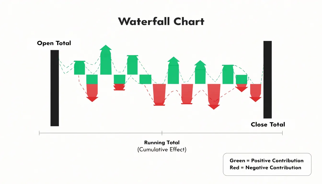
To build one, assemble the data in the exact sequence the changes occurred, since the order shapes both the visual and the narrative. Place the opening balance first and the closing balance last, then calculate a running total after each step. Each intermediate bar spans from the previous cumulative value to the new one, so gains rise from the prior level and losses descend from it. Distinguish increases and decreases with clearly different colors, and use a third neutral color for the start and end totals so the bookends stand out as reference points.
This format suits financial statements that reconcile one period to the next, such as revenue bridges that break down growth drivers and offsets. It also works well for inventory movement, showing opening stock, receipts, shipments, spoilage, and closing stock in a single view. Teams tracking pipelines use it to trace how a starting opportunity value moves through qualification, conversion, and attrition to arrive at a forecast figure. Keep category labels concise, order them logically, and limit the number of steps so the chart remains readable.
Radar Charts
Radar charts, also known as spider charts, compare multiple metrics simultaneously across several entities. Each axis represents a different metric, and values are plotted as points connected by lines to form a polygon, providing an immediate visual summary of an entity’s performance profile. For example, when evaluating job candidates across communication, technical ability, leadership, and creativity, a radar chart displays each candidate’s strengths and weaknesses at a glance. Similarly, in product comparisons, it can show how models stack up on price, battery life, performance, and design, making trade-offs easy to spot.
However, radar charts come with caveats. The visual area of the polygon can be misleading because it depends on the order and scale of the axes; a small change in one metric can disproportionately alter the overall shape. Comparing many entities on the same chart creates clutter, and the layout assumes all axes are equally important and share comparable scales. Therefore, radar charts are best used for a small number of entities and metrics with consistent scales, particularly when the multivariate profile matters more than individual data points, such as in performance reviews, product feature comparisons, and team capability assessments.
Stat Cards
Stat cards serve a single purpose: bringing one high-impact number to the front of the reader’s attention. The number itself should be the largest element in the card, set in a size and weight that clearly outranks every other component. A common approach places the figure in the top-left or centered position, with the label directly beneath it in smaller, muted type. This hierarchy lets a viewer absorb the headline metric in a fraction of a second.
Micro-copy provides the necessary framing. A short, precise label such as “Monthly Active Users” or “Conversion Rate” tells the reader what the number measures, while a secondary line can supply comparison context, for example “vs. last month” or “target: 12,000.” Keep this copy to a handful of words so it does not compete with the number for attention, and use consistent phrasing across a set of cards so viewers can scan and compare them quickly.
Sparklines and trend indicators add movement without clutter. A small inline line chart placed beneath or beside the figure shows direction and volatility at a glance, while a simple up or down arrow paired with a percentage change communicates momentum in an even more compact form. A sparkline suits metrics where the shape of change matters, and an arrow with a delta suits metrics where only the direction is relevant. Use a restrained accent color to distinguish positive from negative movement, reserving stronger color for cases that demand attention.
Color, Labels, and Clutter
Color is one of the fastest channels for communicating information in a chart, and it deserves deliberate choices. Start with a palette built for accessibility: favor combinations that remain distinguishable for readers with color vision deficiencies, such as blue and orange rather than red and green, and ensure colors are perceptually uniform. Maintain sufficient contrast between data marks and the background, and avoid encoding meaning in hue alone, since subtle shades can blur together in print or on small screens. Limiting the palette to a handful of colors keeps the viewer’s attention on the data rather than the decoration.
Labels should sit as close to the data as possible. Direct labeling—placing category names or values next to the marks they describe—removes the need for readers to bounce between a legend and the plot area, speeding comprehension and reducing lookup errors. Annotation is useful for highlighting an important point, though it should be used sparingly so the chart does not become crowded with competing notes.
Gridlines, borders, background fills, and three-dimensional effects often add visual weight without adding information. Stripping these elements away lets the data stand forward and lowers the cognitive effort required to read the chart. Where value axes cannot start at zero, clearly marking axis breaks preserves integrity, and consistent, readable typography rounds out a clean design.
Dashboards
A dashboard is an interactive environment for exploration, and its structural layout determines how easily users can move from a broad overview to a specific question. Begin with a clear spatial arrangement: summary metrics or key performance indicators across the top, primary trends in the central region, and supporting detail panels at the edges or below. This structure gives viewers a predictable starting point and a natural path for drilling deeper. Reserve fixed zones for persistent elements such as date ranges, segment selectors, and navigation, so these controls remain in the same location as the underlying charts change.
Filter controls deserve placement near the data they affect. A region selector positioned directly above a regional sales chart reads more naturally than one tucked into a distant toolbar. Offer sensible defaults so the dashboard opens with a meaningful view, and show active filter states clearly, including the option to reset. Where several charts respond to the same filter, group them visually so users understand the shared scope of their selections.
To keep dynamic views legible, maintain stable category colors across every chart, keep axis scales and units predictable, and use animation sparingly to signal updates rather than to decorate them. Titles and labels should update with the data so viewers always know what they are looking at, and when a filter produces an empty result, display a clear message instead of a blank panel.
Frequently Asked Questions
When should I use horizontal bars instead of vertical bars?
Horizontal bars are the better choice when category names are long, when there are many categories, or when labels would otherwise rotate or truncate along the x-axis. Vertical bars suit a modest number of categories with short labels.
How many lines should I include in a line graph?
Limit the number of lines to what a reader can distinguish at a glance, typically four to six, and use color, line style, or direct end-of-line labels rather than a crowded legend. If series have very different magnitudes, consider a secondary axis with clear labeling or split the chart into small multiples.
How many slices should a pie or donut chart have?
With more than five slices, a pie chart becomes cluttered and labels overlap, so a bar chart or stacked bar chart is often a better choice. The same five-slice rule of thumb applies to donut charts.
How do I choose the right bin width for a histogram?
A useful starting point is to divide the range of values by the square root of the number of observations; for larger or more skewed datasets, a rule based on the interquartile range and cube root of the sample size adapts better. Try two or three neighboring bin widths and compare results, since too few bins compress structure and too many create noise.
How do I fix overplotting in a scatter plot?
Transparency and jittering can reveal where observations concentrate in a dense scatter plot. Use jitter sparingly, since too much displacement can distort the true positions of your data.
Should a choropleth map use raw counts or normalized data?
Normalize choropleth data by population or land area, because raw counts can mislead when larger regions appear more significant simply due to size. Rates, ratios, or percentages are common normalizations, and the choice should match your analytical question.
Tony Astor
Tony writes about data visualization and the tools people use to build charts and dashboards. More about Data Illustrator