How to Aggregate Data for Charts: Sums, Averages and Bins
 By Tony Astor ·
How to Aggregate Data for Charts
Data aggregation for charts combines raw records into summary values—sums for totals, means or medians for typical values, counts for frequency—grouped by category or time interval. Choose the method that matches the question: sums for additive measures, medians for skewed data, and consistent bins or time buckets for distributions and trends.
Table of Contents
Sums
Sums are the most direct aggregation you can apply to a dataset, answering a simple question: what is the total? Adding values across rows produces a cumulative figure that conveys scale, total volume, or overall impact in a single number, without requiring readers to mentally tally individual data points.
Sums work best when underlying values are meaningfully additive. Sales revenue, units shipped, hours logged, and page views all combine naturally into a larger whole, which is often the figure decision-makers care about most. A bar chart showing summed revenue by region lets each region’s total stand on its own while making comparisons between regions immediate. Stacked bars extend this logic by summing category components within a group, so the overall bar height shows the group total while segments reveal the breakdown.
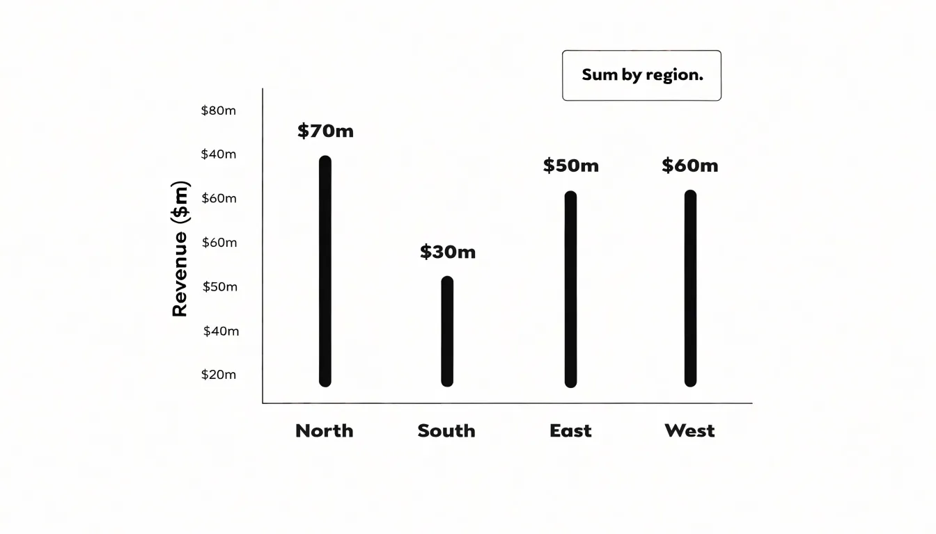
Summing across a dimension collapses detail into a single aggregate, which highlights overall impact but obscures variation inside each group. Choose a grouping level—category, time period, or region—that matches the question being asked. Watch for double counting when rows represent overlapping events, and exclude non-additive fields such as percentages or averages from straight summation. When totals span very different magnitudes, use labels or annotations to keep smaller contributors legible alongside the largest ones.
Averages
Averages describe an entire dataset with a single number representing its typical value. Condensing hundreds or thousands of individual observations into one figure per category—such as average sales per region or average response time per day, plotted as bars or lines—reduces noise and makes trends visible at a glance.
The three main measures of central tendency serve different data shapes:
- Mean: Calculated by dividing the sum of all values by the count of values. It is the most common average and works well when data is roughly symmetric and free of extreme outliers.
- Median: The middle value when data is sorted. Because it is not pulled toward extremes, it is a robust alternative for skewed distributions or datasets with unusually large or small observations. For example, a mean income figure can be distorted by a few very high earners, while median income better reflects what a typical person experiences.
- Mode: The most frequently occurring value, useful for categorical data or for identifying the most common outcome in a set.
Averages also carry a key limitation: they hide the spread of values. Two datasets with the same mean can have widely different underlying distributions. Pairing an average with a measure of variation, such as a range or standard deviation, gives a more complete picture.
Mean vs Median
Because the arithmetic mean includes every observation in its calculation, it is sensitive to every value in the dataset. The median depends on position rather than magnitude—half the observations fall below it and half above—so it responds far less to extreme values.
To choose between them, plot the data as a histogram or sorted view and check for symmetry. A roughly symmetric distribution with no wild values produces a mean and median that sit close together; in that case, the mean is usually the better choice because it incorporates all information in the dataset. When the distribution leans to one side, the two metrics diverge. A long right tail pulls the mean upward and a long left tail drags it downward, while the median stays anchored near the bulk of the observations.
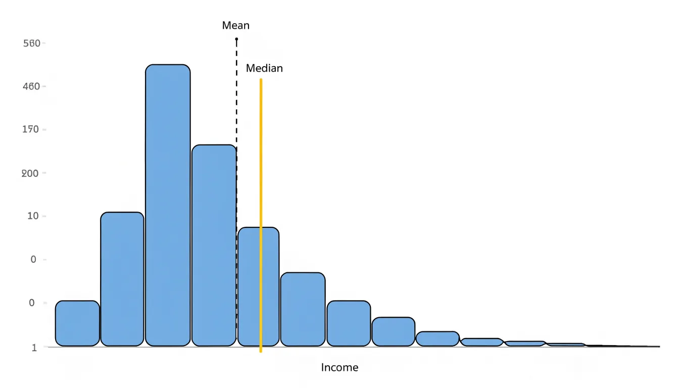
Pay close attention to outliers. A single unusually expensive transaction among typical purchases can shift the mean substantially. If such extremes are genuine and meaningful to the analysis, the mean reflects them honestly. If they are rare anomalies or data errors, the median offers a more stable summary of the typical case.
A useful habit is to compute both and compare them: a large gap signals skew and prompts a closer look. For group comparisons, match the metric to the question. When totals or accumulated values matter, the mean carries more meaning; when describing the typical member of a skewed population, the median gives a fairer picture.
Binning
Binning converts continuous numeric variables—such as thousands of distinct ages, incomes, or response times—into discrete intervals, often called bins or buckets. Assigning each value to a range (such as 0–10, 11–20, 21–30) reduces the number of categories while preserving the overall shape of the distribution. These binned counts or summaries are the foundation for histograms, and they also support grouped bar charts, heat maps, and frequency tables built from numeric data.
The process begins with choosing the width and boundaries of each bin:
- Equal-width bins are the simplest approach and work well when values are spread fairly evenly.
- Unequal or quantile-based bins place roughly the same number of observations in each range, which can reveal structure in skewed data that equal-width bins would hide.
Boundary decisions matter as well: a value sitting exactly on an edge must be assigned consistently to one bin or the other to avoid double counting or gaps.
The trade-off of binning is a loss of detail. Once values are grouped, individual figures are no longer visible, and the choice of bin width can change the impression a chart gives. Testing several bin configurations helps ensure the aggregation communicates the distribution honestly.
Histograms
Unlike bar charts, which compare categorical values, histograms use binned continuous data to show the frequency of observations within each interval. The x-axis shows the variable range divided into bins, and the y-axis shows the frequency or relative frequency of data points falling into each bin.
This structure reveals the distribution’s central tendency, spread, skewness, peaks (modes), gaps, and outliers. For example, a histogram of customer ages might show a concentration of younger customers and a long tail of older ones, informing targeted marketing strategies.
When building histograms, keep bin boundaries clearly defined and consistent, and label both axes with the variable range and frequency measure so the distribution can be interpreted and compared across groups.
Choosing Bin Widths
Bin width determines how much detail a histogram shows and how much structure remains hidden. A width that is too narrow fragments the data into a noisy sequence of spikes, making it hard to separate genuine patterns from random variation. A width that is too wide merges distinct clusters, smooths over gaps, and can conceal secondary peaks, skewness, or outliers.
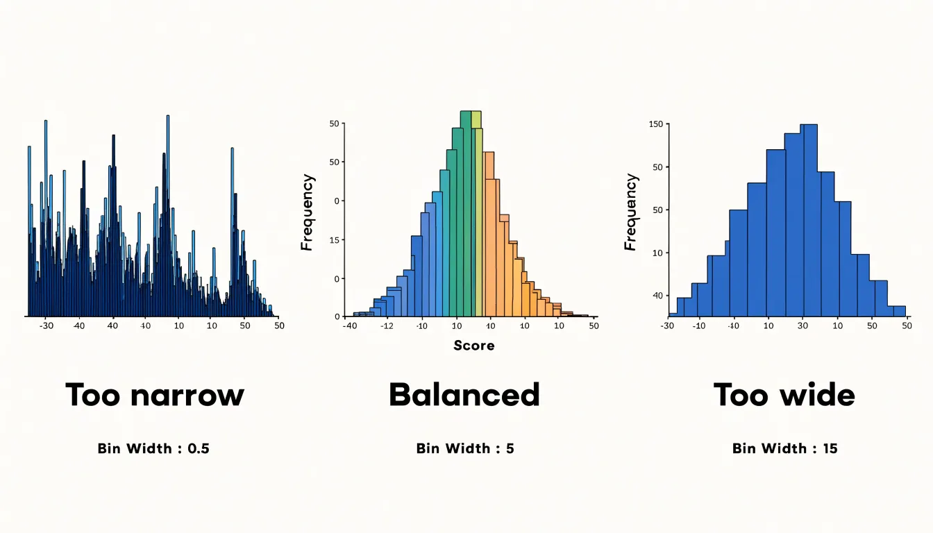
A practical starting point is to divide the data range by between five and twenty bins, depending on sample size. Larger datasets generally justify more bins, while smaller datasets need fewer to avoid sparse, erratic counts. Rule-based formulas such as Sturges’ rule or the Freedman-Diaconis rule offer useful starting points, though they should not be treated as final answers.
The most reliable strategy is iterative visual inspection:
- Generate several versions of the chart with different bin widths and compare them side by side.
- Look for the width at which major patterns remain stable while minor noise disappears.
- Use the exact same bin width when comparing multiple distributions so viewers do not draw false conclusions from differing bin choices.
- Align bin boundaries with round numbers or natural domain thresholds so readers can interpret the bin edges quickly.
Time Series
Time series aggregation groups records with uneven timestamps into consistent intervals such as days, weeks, or months. A daily grouping truncates or floors each timestamp to midnight, a weekly grouping maps each date to the start of its calendar or ISO week, and a monthly grouping assigns records to the first day of their month. This bucketing produces a regular sequence of periods for a chart axis.
Once bucketed, each interval needs an aggregate value matched to the analytical question:
- Sums for counts such as orders or page views.
- Averages for measurements like temperature or response time.
- Minimum or maximum values to identify extremes.
- Last value in the period for cumulative metrics such as account balances, where summing across days would be meaningless.
Intervals with no records should appear as explicit zeroes or nulls rather than being silently dropped, because missing periods create misleading slopes and distort trend lines.
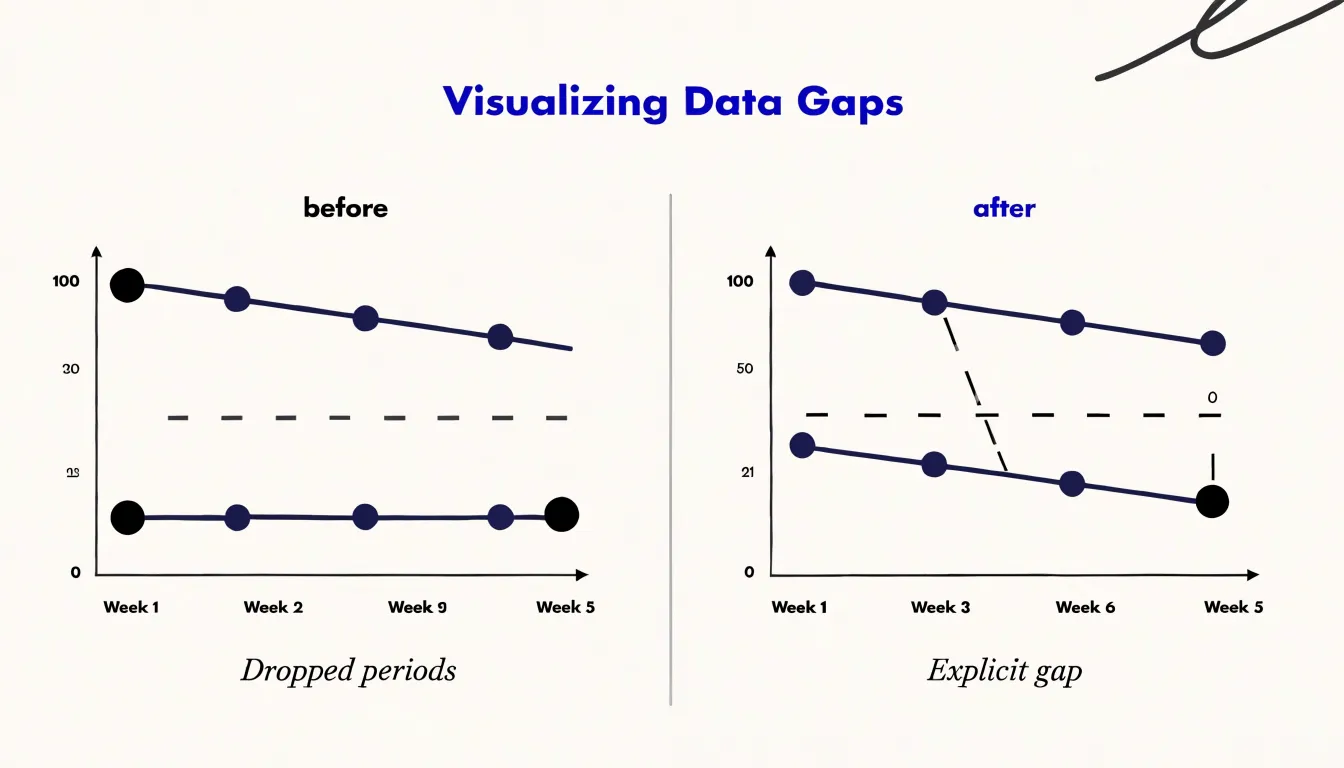
Choosing an interval balances resolution against clarity. Daily aggregation exposes short-term fluctuations and weekday effects; weekly grouping smooths out weekend noise to reveal underlying movement; monthly rollups make seasonality and long-term shifts easier to compare across years. Aligning intervals to calendar boundaries, keeping the aggregation method uniform across the series, and documenting how partial periods are treated keeps time-based charts accurate and comparable.
Handling Null Values
In aggregation, a null is not the same as zero. Most database engines and spreadsheet tools skip nulls entirely during SUM and AVG calculations, while zeroes are included in the math. If a temperature sensor fails for an hour and records zero, the daily average collapses toward an artificially cold figure; if it records null, the average is computed only from the hours with actual readings. Before writing an aggregation query, inspect each column for null counts and determine whether a null represents an unmeasured value, a genuine absence, or a data-entry failure.
The same distinction affects COUNT operations: COUNT(column) ignores nulls, while COUNT(*) includes all rows, so two similar queries can return different totals.
When deciding how to handle nulls in sums and averages, consider the trade-offs of imputation versus explicit display:
- Forward-filling the last known value can work for time series with slow-changing measures.
- Mean substitution is a quick fix, but it shrinks variance and can hide outliers.
- Surfacing missingness directly—by adding a chart note, showing gaps in a line series, or plotting a separate count of null occurrences per period—is often safer.
Apply the same null-handling rules across every chart that shares a dataset. If one dashboard view excludes null regions and another includes them, the numbers will never reconcile. Store null-handling logic in a reusable view or transformation step so every downstream aggregation treats missing values identically.
Grouping Small Categories
When a categorical variable has many low-frequency values, plotting every category creates a cluttered bar or pie chart. Consolidating minor categories into a single “Other” bucket preserves the dataset’s total volume while keeping the focus on major contributors.
Start by examining the frequency distribution and setting a threshold below which categories are merged. For example, if ten product lines each account for less than 2% of total sales, combine them into one “Other” group. The threshold depends on the chart type: pie charts generally work best with no more than five to seven slices, whereas bar charts tolerate more categories before the axis becomes crowded.
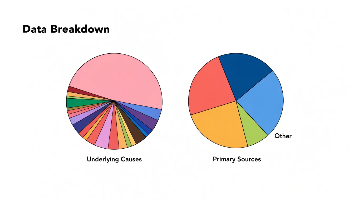
When building the “Other” bucket, sum the underlying values accurately and place the combined category at the end of a sorted bar chart or as the final slice of a pie chart so it reads clearly as a residual group. Document which categories were merged so readers and analysts can trace the consolidation.
Comparing Groups
Presenting totals and means side by side gives a fuller picture of group performance than either metric alone. Totals show overall magnitude and which categories contribute most to the whole, while means normalize for group size so categories with different record counts can be compared fairly. Together, they reveal whether a large total is driven by a high volume of observations or by a high average value.
In a sales dashboard, for instance, one category might generate high total revenue from many small transactions, while another generates lower total revenue from a few large sales. Sorting categories by total highlights volume leaders, while the mean identifies high-value segments with growth potential or high-volume segments that could benefit from upselling.
You can display both metrics using:
- Dual-axis charts, with bars for totals and a line for means (labeled and scaled clearly to avoid confusion).
- Grouped bar charts, with two bars per category.
- Summary tables that place sum and average in adjacent columns for detailed comparison.
Avoiding Common Mistakes
Double counting and skewed ranges are two of the most common aggregation pitfalls, and both can silently distort a chart.
Double counting happens when datasets overlap—such as when a regional sales file shares records with a national summary—or when subtotal rows are mixed in with raw transaction rows. Prevent it by separating raw records from derived summaries in your data model, assigning unique keys, documenting dataset ownership, and deduplicating identifiers across sources before calculating totals.
Skewed ranges occur when bin sizes or time intervals are inconsistent—for example, a bar chart where one bar covers a full year and the next covers a single month. Standardize intervals before grouping by applying a fixed bin width or aligning time buckets to uniform calendar boundaries (such as months or quarters), and label each interval explicitly on the chart.
To catch both errors early, validate aggregates against the source data as a routine step: compare the sum of grouped values with the original record count and total, spot-check a few bins by hand, and scan finished charts for unexpectedly wide bars or unusually large category values.
Matching Metrics to Charts
Each chart type pairs best with specific aggregation methods:
- Bar charts compare discrete categories and pair naturally with sums, averages, or counts per group. Stacked bars and pie charts work well with percentages or part-to-whole sums.
- Line graphs track change across a continuous sequence, usually time. Sum or mean per period is standard, while median or percentile lines work well when the underlying distribution within each period is skewed.
- Scatter plots explore relationships between two quantitative variables. When raw scatter plots are too dense, aggregating to paired group means or medians reduces noise and helps reveal correlation patterns across categories.
Software Shortcuts
Spreadsheets, BI platforms, and databases include built-in tools that automate common aggregations:
- Excel: Functions like
SUM,AVERAGE, andCOUNTsummarize ranges or tables, whileData > Subtotalautomatically groups rows and inserts summary lines. PivotTables let you aggregate large datasets by dragging fields into rows, columns, and values areas. For binning, the Analysis ToolPak provides an automated histogram tool, and theFREQUENCYfunction offers manual control over bin ranges. - Tableau: Dropping a measure onto a shelf applies an aggregation automatically (
SUMby default), which you can change to average, median, count, or other summaries via right-click. TheCreate Binscommand generates equal-width bins from any measure, and Level of Detail (LOD) expressions compute aggregations at custom granularities. - SQL: Aggregate functions (
SUM,AVG,COUNT,MIN,MAX) combined withGROUP BYproduce summary tables directly from the database. Window functions such asSUM() OVER()calculate running totals and moving averages without collapsing rows, while arithmetic expressions likeFLOOR(value/10)*10or theWIDTH_BUCKETfunction handle binning.
Real World Project
To see how cleaning, aggregation, and chart selection fit together, consider a raw transaction table with columns for date, region, product, and sales amount:
- Inspect and clean the raw data: Remove duplicate transaction rows, fill or flag missing values, standardize date formats, and normalize inconsistent region spellings so categories group cleanly.
- Aggregate to match the question: To compare total sales across regions, group the cleaned records by the
regioncolumn and applySUMto theamountcolumn, condensing hundreds of transactions into one summary row per region. - Visualize the summary table: Plot the aggregated table as a bar chart with regions on the x-axis and summed sales on the y-axis, then add data labels, a clear title, and an appropriate axis scale.
Dashboard Overview
Before publishing a dashboard, run through a short checklist for every chart to keep aggregations consistent and trustworthy:
- Data integrity: Confirm the source table has refreshed, row counts match expectations for the reporting period, and nulls or placeholder values are handled consistently. Check for duplicate records, timezone mismatches, upstream rounding, and implausible minimum or maximum values.
- Metric selection: State in one sentence what question the chart answers and verify the chosen aggregation (sum, average, count, or distinct count for unique entities) matches the metric’s meaning. Confirm the data grain matches the chart grain, decide whether totals should roll up or stay segmented, and document the metric definition alongside the visual.
- Chart accuracy: Reconcile aggregated outputs against a trusted source or a manual spot check on a small sample. Verify that axes, labels, units, and time windows match the underlying query, that segmented totals sum to the expected whole, and that dashboard filters interact as intended, noting any exclusions applied during aggregation.
Frequently Asked Questions
When should I use a sum instead of an average in a chart?
Use sums when values are meaningfully additive, such as sales revenue, units shipped, hours logged, or page views, because sums convey total scale, volume, or overall impact. Use averages to describe the typical value per category and reduce noise. Watch for double counting when rows represent overlapping events, and exclude non-additive fields such as percentages or averages from straight summation.
What is the difference between mean and median when data is skewed?
The mean is calculated by dividing the sum of all values by the count and is sensitive to every value, while the median is the middle value when data is sorted. For skewed distributions, a long tail pulls the mean, but the median stays anchored near the bulk of the observations.
How many bins should I use for a histogram?
A practical starting point is to divide the data range by between five and twenty bins, depending on sample size, with larger datasets generally justifying more bins. Use iterative visual inspection and the exact same bin width when comparing multiple distributions.
How should I handle time periods with no data in a time series chart?
Intervals with no records should appear as explicit zeroes or nulls rather than being silently dropped, because missing periods create misleading slopes and distort trend lines.
What should I do with many small categories in a chart?
Consolidate minor categories into a single “Other” bucket to preserve the dataset’s total volume while keeping the focus on major contributors. Pie charts generally work best with no more than five to seven slices, while bar charts tolerate more categories, and you should document which categories were merged.
What is the difference between a null and a zero in aggregation?
A null is not the same as zero; most database engines and spreadsheet tools skip nulls during SUM and AVG calculations, while zeroes are included in the math. Inspect columns for null counts and determine whether a null represents an unmeasured value, a genuine absence, or a data-entry failure.
Tony Astor
Tony writes about data visualization and the tools people use to build charts and dashboards. More about Data Illustrator