Histogram: What It Is and How to Read It
 By Tony Astor ·

Histogram
A histogram is a chart that groups numerical data into consecutive ranges called bins and uses bar height to show how many values fall in each range. Bars touch because the data is continuous, revealing the distribution’s shape, center, spread, peaks, gaps, and outliers. Bar graphs instead display separate categories with gaps between bars.
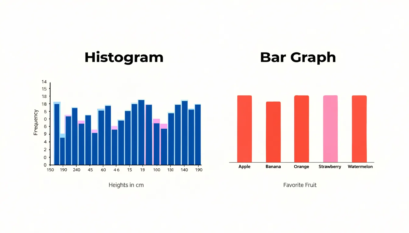
Table of Contents
Histogram
A histogram is a data visualization tool that organizes a collection of numerical values into user-defined ranges, often called bins or buckets, and displays how many data points fall into each range. Each range appears as a bar along the horizontal axis, while the height of that bar reflects the count or frequency of values within that range. The result is a compact picture of how a dataset is distributed, showing where values cluster, where they thin out, and what overall shape the data takes.
Reading a histogram begins with the horizontal axis, which represents the variable being measured, divided into consecutive, non-overlapping ranges. The vertical axis typically shows frequency, meaning the number of observations in each range, though some histograms display relative frequency or density instead. To interpret the chart, look at each bar in turn and ask how tall it is compared with its neighbors. A tall bar signals a range containing many data points, while a short bar indicates a range with few. Gaps between bars show ranges with no observations at all.
The basic structure of a histogram also includes the overall silhouette formed by the bars. A single prominent peak suggests a concentration of values around that range, while multiple peaks point to distinct clusters within the data. A long tail extending to one side reveals a spread of extreme values in that direction. Symmetry or asymmetry in the outline gives a quick sense of how balanced the distribution is.
The choice of range width shapes what the histogram reveals, since wider ranges smooth over detail and narrower ranges expose finer variation. With this basic structure in mind, a histogram becomes an intuitive first look at any dataset, revealing the central tendency, spread, and shape of values before deeper analysis begins.
Histogram vs. bar graph
A histogram and a bar graph can look similar at a glance, yet they serve different purposes and follow different visual conventions. A histogram is designed to display continuous quantitative data, meaning values that can take on any number within a range, such as heights, weights, temperatures, or response times. Because its bins divide a single unbroken numeric scale, the bars are drawn side by side with no space between them. The touching bars signal that the underlying variable flows continuously from one interval into the next, with bins ordered from lowest to highest along the horizontal axis.
A bar graph, by contrast, represents categorical data, where each bar corresponds to a distinct group that has no inherent numeric order, such as types of fruit, brands of cars, or survey response options. Because the categories are separate and discrete, the bars are drawn with noticeable gaps between them. These gaps make clear that the categories stand apart from one another and that the space between bars carries no meaning. In a bar graph, the bars can often be reordered without changing the integrity of the display, since the categories do not follow a continuous scale. Recognizing whether the data is continuous or categorical, and noting whether the bars touch or are separated by gaps, provides a quick way to tell which type of chart is being used and what kind of information it is meant to convey.
Histogram axes
A histogram communicates the distribution of a dataset through two coordinated axes, and reading them correctly is the foundation for interpreting everything the chart shows. On the horizontal x-axis, bins are typically of equal width, so each one corresponds to a specific span of the data, such as test scores between 70 and 80 or heights between 160 and 170 centimeters. The boundaries of each bin matter a great deal: shifting them slightly can change the apparent shape of the distribution, which is why analysts usually choose round, meaningful cut points and state the bin width explicitly. The x-axis values increase from left to right, and adjacent bins share boundaries so that no observation falls between intervals.
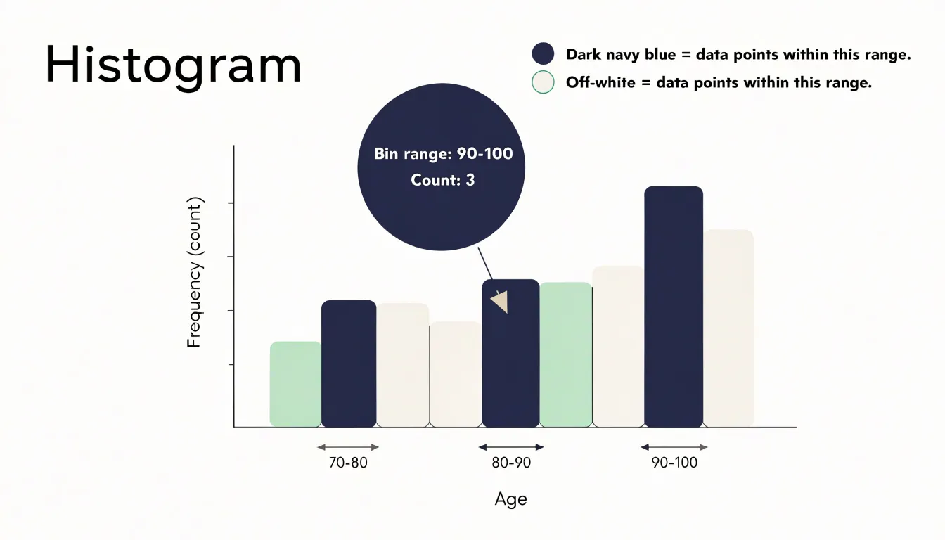
The vertical y-axis records how many observations fall into each bin, either as a raw frequency count or as a percentage of the total. When the y-axis shows counts, the height of each bar tells you exactly how many data points landed in that interval; when it shows percentages or relative frequencies, the heights sum to 100 and make comparisons across datasets of different sizes possible. In some versions the y-axis displays density, where the total area of the bars equals one, which is useful for overlaying smooth curves. Regardless of the scale chosen, the area of each bar is proportional to the number of observations in its bin. Together the axes turn a list of numbers into a shape that reveals peaks, gaps, skew, and outliers at a glance.
Bins and intervals
Bins and intervals form the backbone of any histogram, since they determine how a continuous dataset is transformed into a visual summary. Raw continuous data can take on an enormous number of distinct values within a range, and plotting each individual observation would produce a chart too granular to interpret. Dividing the range into consecutive intervals—such as 0 to 10, 10 to 20, and 20 to 30—covers the full span of the data from the smallest observation to the largest.
The defining property of well-constructed bins is mutual exclusivity combined with collective exhaustiveness. Every data point must fall into exactly one range, and no point may be left out. This is achieved through consistent boundary rules, such as including the lower bound of each interval while excluding the upper bound. A value of exactly 10 would therefore belong to the 10 to 20 bin rather than the 0 to 10 bin, which prevents double counting and ambiguity at the edges. As long as these rules are applied uniformly, each observation is assigned to a single bin, and the sum of the counts across all bins equals the total number of observations in the dataset.
Effective grouping also requires thoughtful choices about bin width and the number of bins. A balanced choice reveals the underlying distribution while keeping the chart readable, and the width should generally be uniform unless there is a strong reason to vary it. Thoughtful binning thus converts a sprawling list of continuous measurements into an interpretable set of counts.
Choosing bin sizes
The choice of bin width is one of the most consequential decisions when constructing a histogram, as it directly influences the shape and interpretation of the distribution. Overly wide bins aggregate too many data points into a single bucket, which can obscure important variations and oversimplify trends. For example, a wide bin might merge two distinct peaks into a single flat mound, hiding the presence of multiple modes. This loss of detail can lead to incorrect conclusions about the underlying data generating process.
On the other hand, overly narrow bins produce a histogram with many small bars, each containing few observations. This introduces noise and makes it difficult to discern the overall pattern. The histogram may appear jagged and erratic, with random fluctuations dominating the visual representation. In such cases, the true distribution is masked by sampling variability.
Selecting an appropriate bin width is a balancing act between smoothing out noise and preserving meaningful structure. Several rules of thumb exist, such as Sturges’ rule or the Freedman-Diaconis rule, which take into account the sample size and spread of the data. However, these are starting points; the analyst should also consider the context and purpose of the visualization. Often, experimenting with multiple bin widths and comparing the resulting histograms can provide deeper insights. Interactive tools allow users to adjust bin width dynamically, facilitating exploration.
Distribution shapes
Recognizing the shape of the underlying distribution is the first step toward understanding what the data are telling you. Common distribution shapes include:
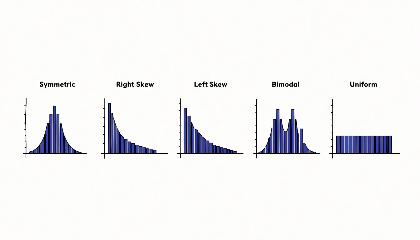
- Symmetric: Looks roughly the same on either side of its central point, with the left and right halves forming near mirror images. The classic bell curve is the most familiar symmetric shape: values cluster around a central peak and taper off gradually toward both tails, a pattern often associated with naturally occurring measurements such as heights or measurement errors.
- Right-skewed: The bulk of the observations sit toward the left and a long tail stretches out to the right, as happens with incomes or waiting times, where a few unusually large values pull the tail outward.
- Left-skewed: Reverses this picture, piling most values on the right with a tail extending toward the lower end, common in data such as exam scores where most students perform well but a handful score very low.
- Bimodal: Shows two distinct peaks separated by a dip, suggesting the data may combine two different groups, for instance the heights of men and women plotted together.
- Uniform: Presents bars of roughly equal height across the entire range, indicating that values are spread evenly with no particular region favored.
Reading these patterns requires attention to the height of the bars, the position of the tallest bars, and the length and direction of the tails. Together these features let you classify a distribution quickly and choose appropriate summary statistics, since measures like the mean and standard deviation behave differently depending on whether the data are symmetric, skewed, or multi-peaked.
Outliers
Outliers are data points that differ significantly from the rest of the dataset, and recognizing them is a key step in data analysis. In a histogram, outliers often appear as isolated bars separated from the main cluster by a gap, or as extreme values at the far ends of the distribution. These unusual points can signal anomalies, data entry errors, or rare but meaningful occurrences. For example, a single bar far to the right might indicate a legitimate but uncommon event, such as a large transaction in a financial dataset, or it could result from a typo like an extra zero.
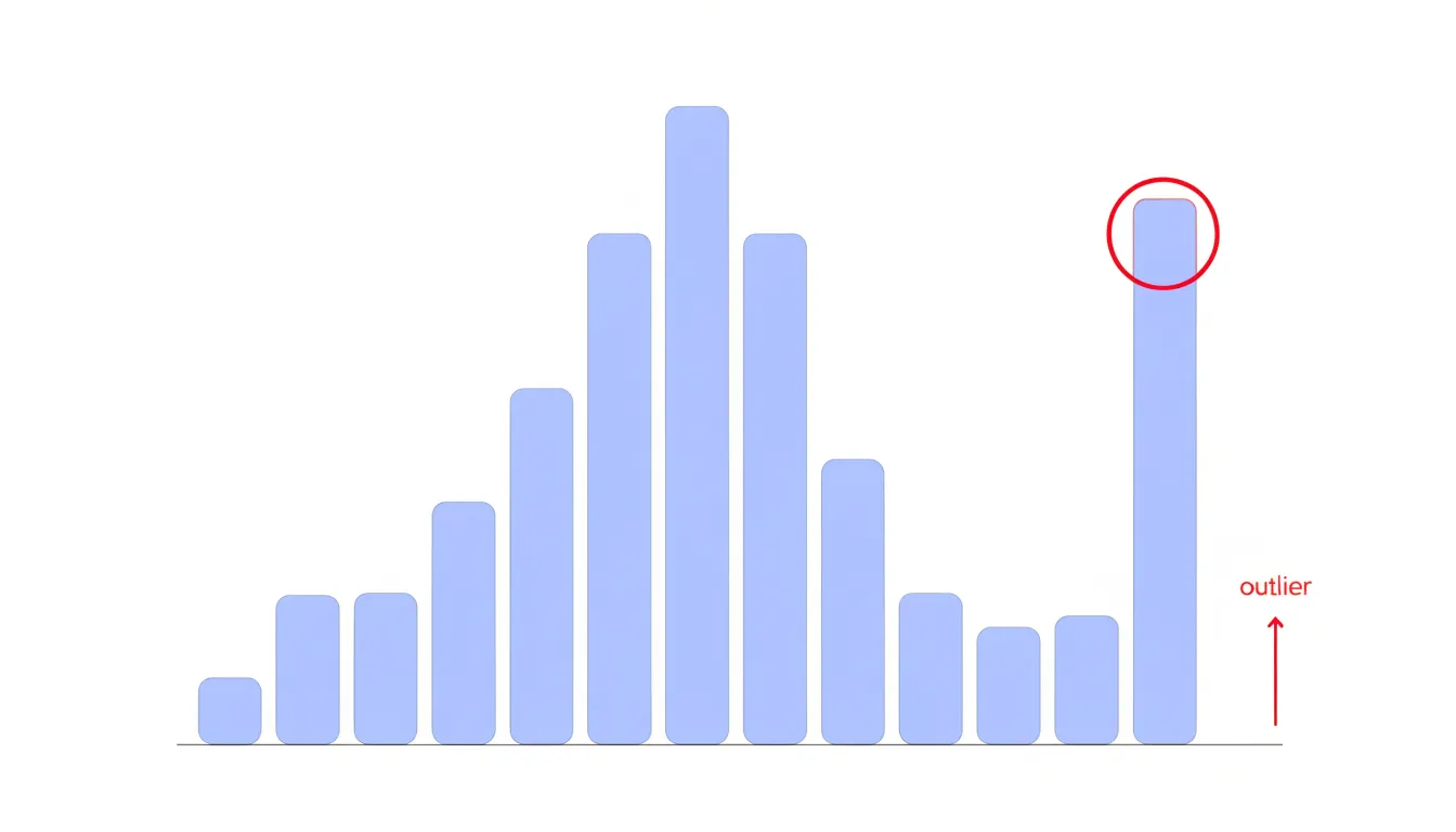
Detecting outliers involves both visual inspection and statistical techniques. Visually, look for bars that are detached from the main body of the histogram or for long tails that stretch far beyond the typical range. Gaps in the histogram can also be telling: a sudden drop in frequency followed by a few isolated bars suggests a distinct subgroup or errors. Statistically, you can use methods like the interquartile range (IQR) rule, where values beyond 1.5 times the IQR from the quartiles are flagged, or z-scores, which measure how many standard deviations a point is from the mean. However, because histograms bin data, outliers may be combined into a single bar; consider adjusting bin widths or using a box plot alongside the histogram for clarity.
Once identified, outliers should be investigated: they might be removed if they are errors, or they might be retained and studied if they represent genuine rare events. Proper handling of outliers ensures that summary statistics and models are not unduly influenced by extreme values, leading to more accurate insights.
Real-world uses
Histograms appear throughout daily life and business to turn raw measurements into a clear picture of typical cases, spread, and exceptions:
- Retail and marketing: Retailers group shoppers into age brackets to see whether the core audience skews young, middle-aged, or older. Marketing teams plot spending data, purchase frequency, or basket size to spot common customer profiles and outliers worth investigating.
- Manufacturing: Quality control engineers plot measurements such as part dimensions, weight, or tensile strength against tolerance limits to see at a glance whether a process is centered, drifting, or producing too many defects near the specification edges.
- Healthcare: Hospitals and clinics chart patient wait times, blood pressure readings, or lab results, helping administrators identify bottlenecks and clinicians recognize unusual patterns.
- Education and human resources: Schools examine test score distributions across classes or years, while HR departments chart tenure, salary bands, or employee satisfaction scores.
- Logistics: Firms track delivery times and package weights to optimize routes and warehouse layouts.
- Finance: Analysts display returns, transaction amounts, or credit scores to assess risk and segment clients.
- Web analytics: Dashboards include histogram-style charts of session durations or page load times to guide performance improvements.
- Personal decisions: Someone comparing apartment rents, commuting distances, or gym visit frequencies can sketch a histogram on paper to see where most values cluster.
Photography histograms
A photography histogram is a graphical representation of the tonal distribution in an image, mapping the brightness of every pixel from pure black on the left to pure white on the right. Digital cameras generate these histograms in real time, allowing photographers to assess exposure accuracy before and after capturing a shot. The horizontal axis represents luminance levels, typically divided into 256 steps for 8-bit images, while the vertical axis shows the number of pixels at each brightness level.
A well-exposed image often displays a bell-shaped curve with data spread across the midtones and tapering toward the extremes. When the histogram shows a spike at the far right, it indicates clipped highlights—areas where pixel values have reached maximum brightness and detail is irrecoverably lost. Conversely, a spike at the far left signals crushed shadows, where detail is lost in darkness. By monitoring the histogram, photographers can adjust exposure settings to shift the tonal distribution, preserving details in both highlights and shadows. For instance, reducing exposure when highlights are clipping brings the rightmost data back into range, while increasing exposure lifts shadow details above the noise floor.
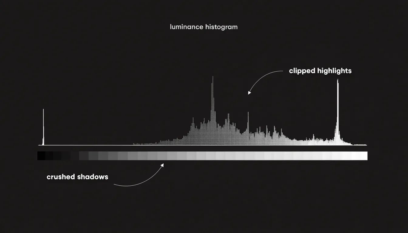
Many cameras also offer RGB histograms, which display separate curves for red, green, and blue channels, helping to detect color channel clipping that might not be obvious in the luminance histogram. Reading these charts empowers photographers to balance exposure and retain maximum tonal information so the final image can be further processed with flexibility.
Healthcare data
Histograms serve as a fundamental analytical tool in healthcare data management, particularly when tracking health trends across populations and within clinical settings. Epidemiological studies frequently employ histograms to visualize the distribution of blood pressure readings across large patient cohorts. By grouping systolic and diastolic measurements into defined intervals, researchers can quickly note whether readings cluster around normal ranges or skew toward hypertensive values. This visual summary helps public health officials recognize shifting patterns in cardiovascular risk across communities and time periods.
In clinical research, histograms of age demographics provide essential context for understanding study populations. Investigators can examine whether participants cluster in particular age bands, which informs the generalizability of trial results and highlights potential gaps in representation. Age distribution histograms also support stratified analyses, allowing researchers to compare treatment outcomes across generational groups.
Symptom onset timelines represent another critical application. During outbreak investigations, epidemiologists plot the frequency of symptom onset dates on a histogram to visualize the epidemic curve. The shape of this curve, whether unimodal or multimodal, offers clues about transmission patterns, exposure windows, and the effectiveness of interventions. Public health teams use these histograms to identify peaks in case reporting, estimate incubation periods, and allocate resources to affected regions.
Beyond these specific use cases, histograms support ongoing quality improvement in hospital settings by revealing patterns in patient vital signs, laboratory results, and length of stay. When combined with statistical process control methods, histogram analysis enables clinicians and administrators to detect anomalies early and respond to emerging health threats with evidence-based strategies.
Step-by-step guide
A consistent four-step procedure gives you a reliable path through any histogram, regardless of the data it represents:
- Begin with the axes. Read the horizontal axis carefully to understand what variable is being measured and what the bin widths represent. Equal bin widths make comparison straightforward, while unequal widths can distort the visual impression of frequency. Then examine the vertical axis to confirm whether it shows raw counts or relative frequencies, since this affects how you describe the height of any bar.
- Identify the central peak. Look for the tallest bar or cluster of bars, which indicates the most common range of values, and note whether a single dominant peak exists or whether several peaks appear. The location of the peak relative to the overall range tells you where the data concentrates.
- Note the spread. Observe how far the bars extend to the left and right, whether the distribution stretches further in one direction, and how quickly the frequencies taper toward the edges. This gives a sense of variability and helps you judge whether values cluster tightly or scatter widely.
- Check for anomalies. Scan for isolated bars standing apart from the main body of data, gaps where no observations fall, or sudden jumps in height. These features may signal outliers, missing values, or distinct subgroups within the dataset.
Common mistakes
Misleading histograms often arise from a small set of recurring design errors that distort the shape of a distribution and lead viewers toward false conclusions:
- Unequal bin widths: When intervals vary in size while the vertical axis still shows raw counts, wider bins naturally accumulate more observations and appear as tall bars, implying a peak that reflects the bin’s span rather than any real concentration of data. The safest remedy is to keep bins uniform, or to plot density rather than counts so that each bar’s area remains proportional to the frequency it represents.
- Truncating the y-axis: Starting the vertical scale above zero exaggerates differences between bars, making modest counts look dramatic and small variations appear as sharp peaks or gaps. For count-based histograms, the vertical axis should generally begin at zero so that the relative heights of bars remain visually honest and the reader can judge proportions at a glance.
- Treating a categorical variable as continuous: Histograms are built for quantitative data measured on an interval or ratio scale, where bin edges mark ranges of real numeric values. Applying this format to discrete categories, such as types of product or departments, suggests an ordering and a continuity between bars that do not exist. In these cases a bar chart is the appropriate choice.
Software and tools
Several widely used software packages make it straightforward to move from raw numbers to a finished histogram:
- Microsoft Excel: Offers one of the most accessible entry points. Its Analysis ToolPak includes a dedicated histogram tool, and newer versions provide a built-in chart type that bins data automatically. For users working with smaller datasets or quick exploratory checks, this low barrier to entry means a histogram can be produced in a few clicks, with adjustable bin widths and axis labels available directly in the chart formatting menus.
- Python (Matplotlib): Serves analysts who need programmatic control and reproducibility. The
pyplot.histfunction accepts an array of values plus parameters for the number of bins, range, and normalization, so a script can regenerate the same figure whenever the underlying data changes. This suits workflows involving automated reporting or large datasets that would be unwieldy to handle by hand. - R: Provides comparable capability through its base
histfunction and through ggplot2’sgeom_histogram. The tidyverse ecosystem makes it easy to group data by category and produce faceted histograms that compare distributions side by side, which is valuable for statistical exploration before formal modelling. - Tableau: Occupies the business-intelligence end of the spectrum. Users drag a continuous measure onto a shelf and Tableau generates a histogram, with bin size adjusted through a slider or a calculated field. Its strength lies in interactive dashboards, where filters and tooltips let viewers explore the shape of a distribution without writing code.
Across all four tools, sensible defaults handle much of the setup, while options for bin counts, axis scaling, and labelling allow the chart to be tuned for clarity. Choosing among them depends largely on the size of the dataset, the need for repeatability, and whether the audience will view a static image or interact with the chart directly.
Summary statistics
Summary statistics provide a numerical bridge between the visual shape of a histogram and the underlying data distribution:
- Mean: The average, or the balance point where the histogram would balance if the bars were physical weights. In a symmetric, bell-shaped histogram, the mean sits at the center of the peak. When the distribution is skewed, the mean is pulled toward the long tail, because extreme values exert a strong influence on the sum.
- Median: The middle value when data are ordered, corresponding to the vertical line that divides the total area of the histogram into two equal halves. In a skewed distribution, the median remains closer to the bulk of the data and is less affected by outliers, so it often lies between the mean and the mode.
- Mode: The most frequent value, represented by the tallest bar in the histogram. In a perfectly symmetric unimodal distribution, mean, median, and mode coincide at the center. In a right-skewed distribution, the mode is the smallest of the three, the median is intermediate, and the mean is largest; in a left-skewed distribution, the order reverses.
- Standard deviation: Measures the spread of the data around the mean. On a histogram, a small standard deviation produces a narrow, tall peak, while a large standard deviation yields a wide, flat distribution. In a roughly normal distribution, about 68% of values fall within one standard deviation of the mean, and about 95% within two.
These summary statistics translate the visual features of a histogram—peak location, tail length, and overall width—into precise numerical descriptions that guide interpretation and comparison across datasets.
Overview
When you collect hundreds or thousands of observations, individual values blur together and patterns become invisible. Beyond simple description, the histogram functions as a diagnostic instrument that makes this invisible structure visible before any formal modeling begins. Its observations guide the choice of statistical methods, flag potential outliers, and suggest whether a data transformation might be needed. In exploratory research, it can reveal hidden subgroups that merge into a single blended population, while keeping the display approachable for audiences without statistical training.
The enduring value of the histogram lies in its ability to capture distributional details that summary statistics alone can obscure. Two datasets can share an identical mean and standard deviation while possessing entirely different shapes, and only the histogram makes that difference immediately apparent. By compressing raw numbers into a coherent visual form, it lets practitioners spot patterns, generate hypotheses, and communicate findings with clarity.
Frequently Asked Questions
What is a histogram and what does it show?
A histogram is a data visualization tool that organizes numerical values into user-defined ranges, often called bins or buckets, and displays how many data points fall into each range. Each bar represents a range, and the height of that bar reflects the count or frequency of values within that range.
How is a histogram different from a bar graph?
A histogram displays continuous quantitative data, with bars drawn side by side with no space between them because the underlying variable flows continuously from one interval into the next. A bar graph represents categorical data, with noticeable gaps between bars because the categories are separate and discrete.
How do I choose the right bin size for a histogram?
Overly wide bins can obscure important variations and oversimplify trends, while overly narrow bins introduce noise and make the overall pattern difficult to discern. Selecting an appropriate bin width is a balancing act, and rules of thumb such as Sturges’ rule or the Freedman-Diaconis rule can be starting points, but the analyst should also consider the context and purpose of the visualization.
What do different histogram shapes mean?
Common distribution shapes include symmetric, right-skewed, left-skewed, bimodal, and uniform. A single prominent peak suggests a concentration of values around that range, multiple peaks point to distinct clusters within the data, and a long tail extending to one side reveals a spread of extreme values in that direction.
How can I spot outliers in a histogram?
Outliers often appear as isolated bars separated from the main cluster by a gap, or as extreme values at the far ends of the distribution. Visually, look for bars detached from the main body of the histogram or long tails that stretch far beyond the typical range, and statistically you can use methods like the interquartile range rule or z-scores.
What does a photography histogram show?
A photography histogram is a graphical representation of the tonal distribution in an image, mapping the brightness of every pixel from pure black on the left to pure white on the right. A spike at the far right indicates clipped highlights, while a spike at the far left signals crushed shadows.
Tony Astor
Tony writes about data visualization and the tools people use to build charts and dashboards. More about Data Illustrator