Histogram vs Density Plot: Bins or Curves?
 By Tony Astor ·

Histogram vs Density Plot
A histogram plots exact counts of data in fixed-width bins, so bar heights sum to the sample size and boundaries, gaps, and outliers stay visible. A density plot applies kernel density estimation to draw a smooth continuous curve whose area equals one, showing overall shape, skew, and multiple modes without depending on bin edges.
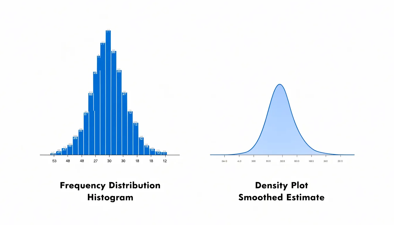
Table of Contents
Histogram
A histogram begins with a simple act of classification: dividing the full range of a continuous variable into a series of adjacent intervals, commonly called bins. Each bin defines a distinct segment of the data, such as values between 10 and 20 or between 20 and 30, and every observation in the dataset is assigned to exactly one of these segments. Once the assignment is complete, the histogram counts how many observations fall into each bin and represents that count as the height of a bar. The result is a compact summary of exact frequencies across clearly defined ranges, which makes it straightforward to see where the bulk of the data sits, how spread out the values are, and whether the distribution skews toward one end.
Because the bars are contiguous and the bin edges are fixed, the height of each bar corresponds directly to a count rather than a probability density, so totals can be recovered by summing bar heights. This property makes histograms especially useful for exploratory work, quality checks, and communicating volume alongside shape.
The mechanics also involve decisions about bin width, bin boundaries, handling values that land exactly on an edge, and whether to use equal-width or custom intervals. Those choices determine how faithfully the histogram reproduces the underlying data structure. In practice, a well-constructed histogram turns thousands of raw measurements into an interpretable profile of counts across ordered ranges, providing a foundation for comparison, anomaly detection, and further statistical analysis.
Density Plot
A density plot visualizes the distribution of a dataset by drawing a smooth curve across the range of observed values. The curve represents the probability density function, giving a continuous picture of where values are concentrated and how they spread across the number line. The transformation from raw observations to that smooth curve relies on kernel density estimation, or KDE, a technique that builds the curve directly from the individual data points.
Kernel density estimation works by placing a small, symmetrical bump, called a kernel, at the position of every data point. Common kernel shapes include the Gaussian bell curve and the Epanechnikov function. Each kernel represents a localized contribution to the overall distribution, centered on one observation. Where many data points cluster together, their overlapping kernels stack up and produce a taller, denser region of the curve. Where observations are sparse, the kernels are isolated and the resulting curve remains low.
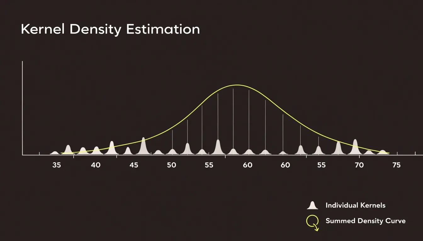
The heights of all these overlapping kernels are summed at every point along the horizontal axis, and the total is normalized so that the area under the final curve equals one. This normalization turns the accumulated bumps into a proper probability density function. The result is a single continuous line that captures the shape of the data: peaks indicate common values, valleys indicate gaps, and the tails show how far the values extend in each direction.
The smoothness of the curve depends on a parameter called the bandwidth, which controls the width of each kernel. Choosing an appropriate bandwidth balances detail against clarity, and the smooth curve that emerges makes it easy to compare distributions and identify features such as skew, multiple modes, and overall spread.
Bin Width
Bin width is the single most consequential choice when constructing a histogram, because it determines the granularity at which the data’s structure becomes visible. The width of the intervals acts like the resolution setting on a lens: adjust it, and different features of the same dataset come into focus or dissolve into noise.
When bin intervals are set too narrow, each bar covers a tiny slice of the value range, and the resulting chart tends to fragment into a jagged, erratic skyline. Small counts per bin make the shape highly sensitive to random fluctuations, so sampling noise dominates the picture. Genuine trends, such as a smooth unimodal peak or a gentle skew, become difficult to perceive because the eye is drawn to spurious spikes and gaps that reflect chance rather than structure.
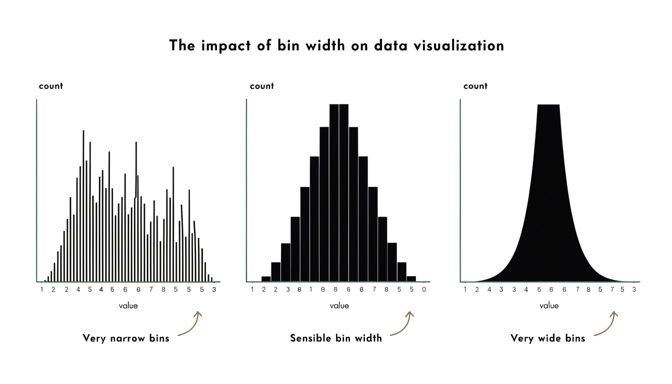
When bin intervals are set too wide, the opposite distortion occurs. Each bar aggregates a broad stretch of values, and distinct clusters, secondary modes, or sharp cutoffs within that stretch are merged into a single block. A dataset with two separate subgroups can appear as one bland lump, and the precise location of a boundary or threshold disappears. Wide bins produce a tidy but misleadingly smooth profile.
A useful working rule is to try several bin widths and compare the resulting shapes. Stability across a range of widths suggests that the features are real; features that appear only at one particular setting are likely artifacts of the binning choice. Sturges’ rule and Scott’s rule offer algorithmic starting points based on sample size and spread, but visual comparison remains the most reliable guide. Reporting the chosen bin width alongside the chart lets readers judge the histogram’s claims for themselves.
Smoothing
The bandwidth parameter in a density plot determines how widely the kernel spreads the influence of each observation when constructing the estimate. Choosing the right bandwidth is where most of the practical work in density estimation happens, since the curve’s usefulness as a summary of the underlying distribution rises and falls with this setting.
A generous bandwidth produces a curve that averages across large stretches of the data. Peaks flatten, valleys fill in, and the overall outline of the distribution emerges clearly. This is valuable when the analytical goal is to communicate the general shape of the data, to compare broad features across groups, or to present a distribution to an audience that needs a clean visual summary. The risk of this generous setting comes when genuine structure gets swallowed by the averaging, and distinct modes merge into one broad hump.
A narrow bandwidth takes the opposite posture. Each observation influences only a small neighborhood, so the curve follows local fluctuations closely. Fine structure, such as secondary modes and subtle shoulders, becomes visible. The cost of a narrow bandwidth is a curve that reports sampling noise alongside real signal. Small, jagged bumps appear that reflect the particular sample rather than any feature of the population.
The working rule is to examine several bandwidths before settling on one. Comparing an oversmoothed version, an undersmoothed version, and one or two intermediate settings reveals which features persist across settings and which appear only at one extreme. Features that survive a range of bandwidths deserve interpretation. Features that come and go are fragile artifacts of the smoothing choice. Reporting the bandwidth alongside the plot, or showing a small panel of alternatives, gives readers the context to judge the curve for themselves.
Histogram vs Density Plot
A histogram presents data as a stepped skyline of solid blocks butted against one another, with sharp vertical edges and flat tops. A density plot renders the same underlying distribution as a fluid, continuous contour. The histogram reads as something built from discrete units, while the density plot reads as something drawn in a single motion.
That difference in visual texture shapes how each chart is perceived:
- Blocks emphasize boundaries: The eye can trace exactly where one bin ends and the next begins, making it easy to count observations and see the granular composition of the data. However, the skyline changes noticeably when the bin size is adjusted.
- Curves emphasize flow: The eye follows an uninterrupted line, registering peaks, shoulders, and long tails as continuous features rather than as collections of separate columns. A density curve offers a more stable silhouette, though it can soften or obscure fine-grained structure that bars would show plainly.
Choosing between the two comes down to whether the story lives in the individual counts and their hard edges or in the overall shape and its flowing contours.
Data Patterns
Both histograms and density plots reveal where values cluster and how they behave across the range.
- Modality (Peaks and Valleys): Peaks in the data, called modes, indicate the most common values or ranges. A single prominent peak signals a unimodal distribution, while two distinct peaks point to bimodality, often hinting that two subgroups exist within the data. Density plots tend to make these peaks easier to see because a smooth curve highlights the contours, whereas a histogram’s tall bars depend on the chosen bin width. Valleys, the low points between peaks, matter just as much: a deep valley between two modes suggests the groups are well separated, while a shallow valley indicates overlap.
- Skewness: Skewness describes the asymmetry of a distribution. When the tail stretches toward higher values and most observations sit on the left, the data are right-skewed; the reverse holds for left-skewed data. Density curves show this asymmetry fluidly through the direction and length of the tail, and histograms show it through the gradual tapering of bar heights. Recognizing skew helps analysts decide whether summary statistics like the mean will give a misleading picture of the typical value.
- Gaps and Outliers: Gaps appear as empty stretches where no observations fall, visible as blank intervals between histogram bars or as flat regions in a density curve. Such gaps can flag separate populations, data entry issues, or genuine boundaries in the measured phenomenon. Outliers sit at the far edges of the plot as isolated bars or as a thin tail extending well beyond the main body of the curve.
Comparing both plot types side by side gives a fuller picture of modality, skewness, gaps, and extreme values, since each format reveals slightly different features of the same underlying pattern.
Sample Size
Sample size plays a decisive role in whether a histogram or a density plot will communicate your data clearly.
With small samples, a histogram is usually the safer choice. When you have only a few dozen observations, each bin contains just a handful of points, and the resulting bars directly reflect how many values fall into each range. Readers can see the actual counts behind the shape and immediately gauge how much uncertainty surrounds each bar. With sparse data, a density plot’s smoothing has little real information to work with, so the resulting curve can shift dramatically depending on the bandwidth chosen, and it may imply a level of precision the data simply cannot support.
As datasets grow into the hundreds, thousands, or millions of observations, the tradeoff reverses in favor of the density plot. Large samples fill bins densely enough that histogram bar heights become stable, but the sheer number of bins needed to capture detail can make a histogram look noisy and blocky. A density plot smooths across the fine-grained fluctuations, revealing the overall shape in a form that stays readable regardless of sample size.
In practice, small samples benefit from the honest, granular counts of a histogram, while large samples reward the clean, continuous summary a density plot provides.
Overlapping Groups
When a dataset contains several groups, comparing their distributions within the same visual frame is much easier with density plots than with histograms.
In a histogram, when several groups share discrete bins, the bars either cluster or stack on top of one another. Stacking produces a tall column whose total height reflects the sum of all groups rather than the shape of any single group, and overlapping rectangles compete for the same space. A viewer must mentally subtract each layer to recover the original group patterns, which becomes more difficult as the number of groups grows.
Density plots handle this task gracefully. Each group can be drawn as its own smooth curve in a shared plotting area, and by assigning partial transparency to the shaded regions beneath them, the viewer can see where distributions coincide and where they diverge. Because each curve remains a distinct line, groups with small counts are not swallowed by larger ones, and the eye can follow each outline across the full range of the data. This layering makes it easy to spot shifts in central tendency, differences in spread, and the presence or absence of multiple modes across categories. The technique scales comfortably to three or four categories and works well for exploratory analysis, presentations, and reports where the comparative message needs to be read at a glance.
Edge Effects
Kernel density estimation works well when data range freely, but it encounters trouble at boundaries where the variable cannot exist beyond a certain value. A common example is a measurement that cannot be negative, such as income, waiting times, or physical dimensions. When observations cluster near zero, the symmetric kernels centered on those points extend into the negative region. The resulting density estimate therefore assigns positive probability to impossible values below zero. This artifact is known as edge effect or boundary bias.
The distortion is most severe when the bandwidth is large relative to the distance of the nearest observations from the boundary. In such cases, the estimated curve can show a spurious hump just inside the boundary and a misleadingly steep drop at zero, rather than the true shape of the distribution. The problem is not limited to zero bounds; any hard limit, such as a maximum possible score or a physical ceiling, can produce similar leakage. The practical consequence is that summary statistics derived from the curve, such as the estimated mean or the probability of being below a threshold, may be biased.
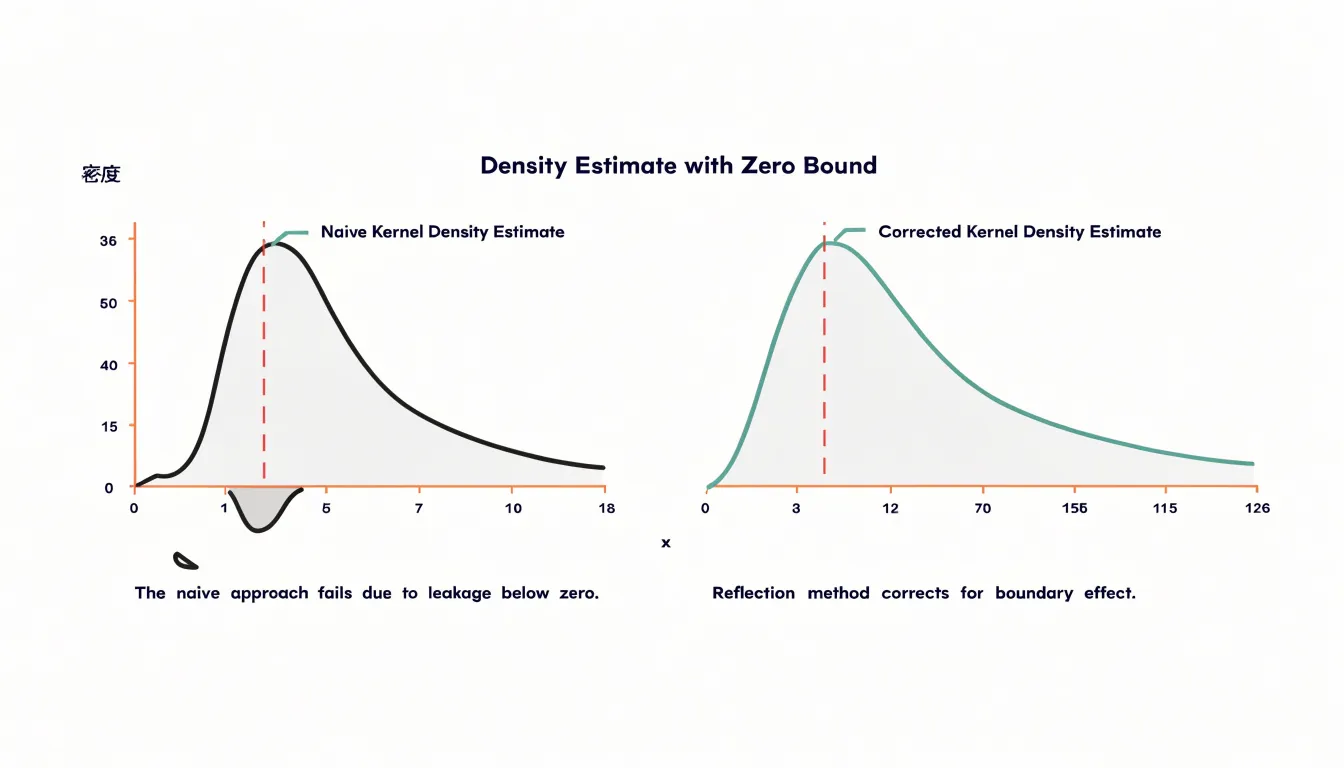
Analysts should recognize when their data have natural boundaries and consider whether standard kernel density estimation is appropriate. Several corrections exist:
- Reflection methods that mirror data across the boundary.
- Boundary kernels that adjust the shape near edges.
- Transformation approaches that map the bounded domain to the real line before estimation.
Without such adjustments, the density plot can misrepresent the data precisely where interest is often highest.
Counts vs Percentages
Reading heights correctly on a histogram or density plot begins with identifying which vertical scale is in use.
- Raw Counts: In a count-based histogram, each bar height reports the number of observations in that bin. A bar reaching 40 means forty data points landed within that interval, and the total across all bars equals the sample size. This makes the chart easy to interpret for a single dataset, since every height is a direct tally of records.
- Percentages or Proportions: When each bar height is divided by the total number of observations, the bars sum to 1 (or 100 percent), and a height of 0.40 means forty percent of the sample occupies that bin. This normalized view allows comparison between datasets of very different sizes, because the scale no longer depends on how many records were collected.
- Probability Density: In a density plot, the curve’s height represents probability density rather than a count or a simple proportion per bin. The area under the curve between two values gives the probability of observing a value in that range, and the total area under the entire curve equals 1. Density values can exceed 1 when the bandwidth is narrow, which surprises readers accustomed to percentages. The key is that height alone is not the probability; the area is.
Always check the axis label and units before interpreting any peak. A tall bar in a count histogram may simply reflect a large sample, while the same shape on a density scale reflects concentration relative to the spread of the distribution. Comparing heights across charts built on different scales leads to false conclusions. Matching the axis to the question—whether absolute frequency or relative probability—keeps the visual reading aligned with the underlying statistic.
Long Tails
Heavily skewed distributions present a real challenge for visualization because the bulk of the data can crowd into a narrow range while a long tail stretches far to one side. In a histogram with fixed bin widths, if the bins are sized to capture the extreme values, the main body of the data compresses into a few tall bars and subtle features inside that mass disappear. If the bins are sized for the dense region, the tail may be reduced to a single bin or vanish entirely. Density plots face a related difficulty, since a kernel bandwidth that smooths the central peak nicely can flatten minor clusters into undifferentiated bumps along the tail.
Several techniques help keep both ends of the distribution visible:
- Logarithmic scaling: Transforming the horizontal axis spreads out the long tail and brings distant extreme values into view alongside the central mass.
- Variable-width or adaptive binning: Histograms can allocate more resolution where the data is dense and broader bins where it thins out.
- Bandwidth adjustment or scale transformation: For density plots, adjusting the bandwidth or plotting on a transformed scale can reveal small secondary clusters that would otherwise be smoothed away.
These choices matter most when the tail is the story, as with income data, response times, or file sizes, where rare but extreme values carry important meaning. By transforming axes or adapting bin widths, the visualization preserves the prominent peak while keeping minor clusters and extreme observations visible and interpretable.
Combined Plots
Overlaying a density curve on top of a histogram brings two complementary views of the same data into a single frame. The histogram provides the empirical foundation of actual counts and empty ranges, while the density line traces the smoothed continuous profile across the full range of values.
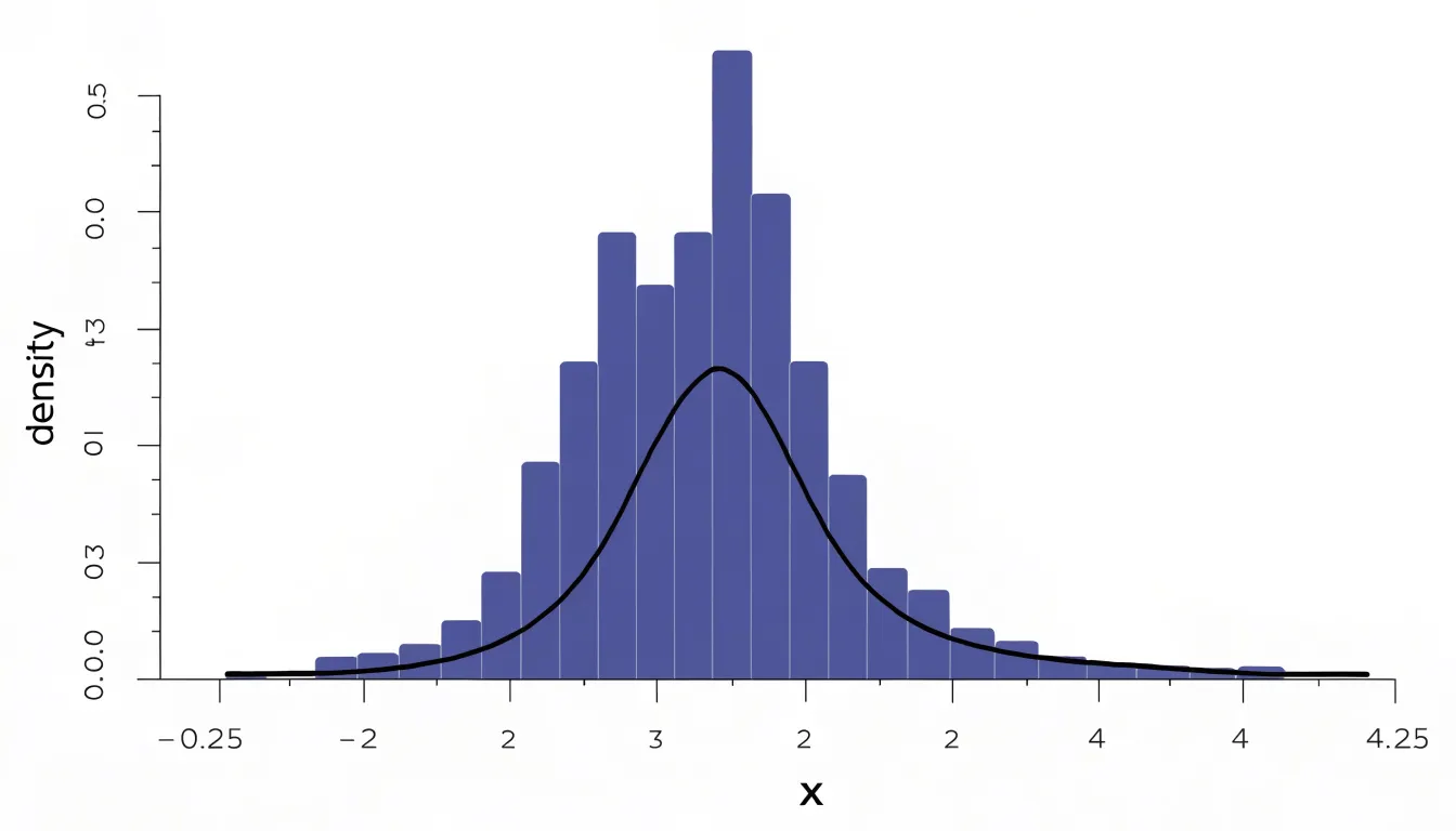
Building a combined plot usually starts with the histogram, after which a kernel density estimate is computed from the same observations and drawn as a line across the bars. A practical detail is scale alignment: histograms can be drawn with raw counts on the vertical axis or with densities that integrate to one, and the curve should match whichever convention is chosen. Many plotting libraries handle this automatically when a density argument is enabled, drawing bars as proportions so the line sits naturally over them.
The pairing is useful in exploratory work because each element compensates for the limits of the other. Seen together, the bars anchor the curve to observed frequencies, and the curve fills in the silhouette between and beyond the bins. The result is a compact summary that serves both readers who want to know how much data lies in each range and readers who want an immediate sense of the overall form of the distribution.
Decision Guide
Choosing between a histogram and a density plot is easier when you evaluate four practical factors:
- Analytical Goal: Use a histogram to show exact counts within defined intervals, reveal gaps or irregular spikes, or let readers estimate frequencies directly. Use a density plot to convey the overall shape of a distribution or to compare several overlapping groups on one set of axes.
- Sample Size: Use a histogram for small samples so the raw structure and uncertainty remain visible. Use a density plot for large samples where a continuous summary is cleaner than dozens of blocky bars.
- Audience: General audiences are accustomed to bars and can interpret a histogram with little explanation, while density curves may need a brief introduction. Technical or statistical audiences often expect the smooth comparison that density plots provide.
- Medium and Size: Dense histograms with many bins can render poorly at small sizes, whereas smooth curves scale down gracefully in slide decks and dashboards.
As a rule of thumb, begin with a histogram to explore the data, then adopt a density plot when comparison and shape are the central message.
Dashboard Overview
Clear charts in reporting dashboards depend on deliberate choices about labels, colors, and scales.
- Labels and Titles: Labels should sit close to the data they describe, use plain language, and include units so readers never have to guess what a number represents. Axis titles belong on every chart, and tick labels should be sparse enough to read at a glance without crowding the plot area. Chart titles should state the takeaway directly rather than naming the chart type, giving viewers an immediate orientation to what they are seeing.
- Color: A restrained palette with a single accent for the most important series keeps attention where it belongs, while consistent color assignments across a dashboard let viewers track the same category from one chart to the next. Sequential and diverging palettes suit ordered or directional data, and colorblind-safe combinations protect readability for every audience. Gridlines and backgrounds should recede into light neutrals so the data marks stay visually dominant.
- Scales: Starting a bar chart axis at zero preserves honest comparisons of magnitude, while line charts tracking change over time can use a tighter range when the variation matters more than the absolute level. Consistent scales across related charts prevent misreading, and logarithmic scales should be labeled explicitly when they appear. Density curves and histograms on the same dashboard benefit from matching axis ranges so viewers can compare shapes directly. Limiting the number of tick marks, rounding values to meaningful precision, and annotating key thresholds or events helps viewers interpret scale changes without extra explanation.
Frequently Asked Questions
What is the difference between a histogram and a density plot?
A histogram shows data as contiguous bars whose heights reflect counts in fixed bins, while a density plot shows a smooth curve representing probability density. Histograms emphasize boundaries and exact counts, while density plots emphasize continuous shape and flow.
How do I choose the right bin width for a histogram?
Bin width determines the granularity of the histogram, and the article recommends trying several widths and comparing the resulting shapes. Features that remain stable across widths are more likely real, while features that appear at only one setting are likely binning artifacts. Sturges’ rule and Scott’s rule can provide starting points, but visual comparison is the most reliable guide.
How do I choose the bandwidth for a density plot?
Bandwidth controls how widely each kernel spreads each observation’s influence. A generous bandwidth gives a cleaner general shape but can merge distinct modes, while a narrow bandwidth reveals fine structure but also sampling noise. Examine several bandwidths and interpret features that persist across settings.
Should I use a histogram or density plot for small samples?
With small samples, a histogram is usually the safer choice because its bars directly reflect how many values fall into each range, and readers can gauge uncertainty. A density plot’s smoothing has little real information to work with in sparse data and may imply more precision than the data support.
How do density plots handle overlapping groups?
Density plots can draw each group as its own smooth curve in a shared plotting area, and partial transparency under the curves helps show where distributions coincide or diverge. This keeps groups with small counts from being swallowed by larger ones and scales comfortably to three or four categories.
What are edge effects in kernel density estimation?
Edge effects, or boundary bias, occur when data have a natural boundary and symmetric kernels extend beyond it, so the density estimate assigns positive probability to impossible values. The distortion is most severe when bandwidth is large relative to the distance of nearby observations from the boundary. Adjustments include reflection methods, boundary kernels, and transformation approaches.
Tony Astor
Tony writes about data visualization and the tools people use to build charts and dashboards. More about Data Illustrator