Histogram vs Box Plot: Which Shows a Distribution Better?
 By Tony Astor ·

Histogram vs Box Plot
A histogram plots continuous data in adjacent bins, with bar height showing the frequency of values in each interval, revealing shape, spread, and multiple peaks. A box plot summarizes data using five numbers—minimum, Q1, median, Q3, and maximum—showing the interquartile range and flagging outliers beyond 1.5×IQR.
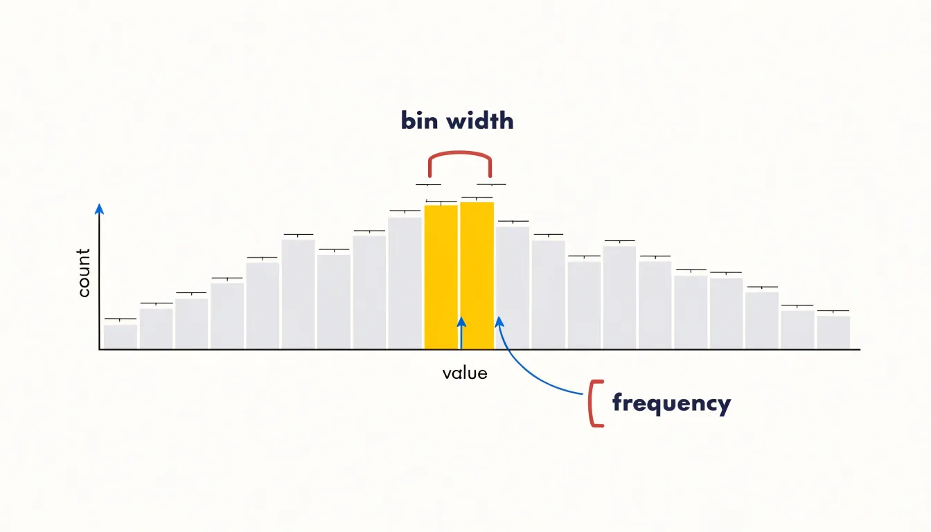
Table of Contents
Histogram
A histogram visualizes the distribution of continuous data by dividing the entire range of values into adjacent intervals, often called bins, and counting how many data points fall into each one. This binning process transforms raw, continuous measurements into a discrete set of frequency counts, showing the overall shape and spread of the data at a glance. Once the bins are defined, each bar represents an interval, with its height proportional to the number of observations inside it.
The choice of bin width is critical: too few bins can oversimplify the distribution and hide important details, while too many can produce a noisy plot that obscures the underlying pattern. Typically, analysts experiment with different bin widths or use rules such as Sturges’ formula or the Freedman-Diaconis rule to select an appropriate number of bins.
This visual representation allows viewers to quickly identify key features of the distribution, including its central tendency, variability, skewness, and the presence of multiple peaks or outliers. Because histograms aggregate data, they are particularly useful for large datasets where individual values are too numerous to examine separately. They provide a compact summary of the data’s frequency structure, enabling comparisons across different groups or time periods. In practice, histograms are widely used in exploratory data analysis, quality control, and statistical inference to assess assumptions such as normality.
Box Plot
A box plot summarizes a dataset using five key numbers—often called the five-number summary—that capture the distribution’s shape and spread:
- Minimum: The lowest observation.
- First quartile (Q1): The value below which roughly a quarter (25%) of the observations fall.
- Median (Q2): The midpoint that splits the dataset into two equal halves (50% below, 50% above), offering a measure of central tendency that resists distortion from extreme values.
- Third quartile (Q3): The value below which roughly three quarters (75%) of the observations fall.
- Maximum: The highest observation.
These five numbers translate directly into the plot’s geometry. The first and third quartiles form the edges of a rectangular box, and a line drawn across the box at the median shows where the middle of the data lies. The height or length of the box, known as the interquartile range (IQR), contains the middle 50% of the data and indicates how tightly the central half is packed. A compact box signals consistency, while a tall or long box signals wide variability among typical observations.
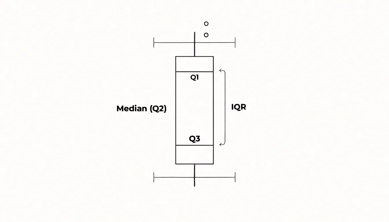
Lines, often called whiskers, extend from the box toward the minimum and maximum, or toward the most extreme values within a defined range when outliers are plotted separately. The five-number summary makes box plots valuable for fast statistical comparison. Analysts can read the center, spread, and skew of a distribution at a glance, then place several box plots side by side to compare groups on a common scale. This compactness suits large datasets and dashboards where space is limited, since a single small graphic conveys the essential structure of hundreds or thousands of values.
Histogram
Reading a histogram begins with the silhouette of its bars, which encodes the distribution’s underlying structure. Start by scanning the tallest bars to locate the modal peaks—the values where observations cluster most densely:
- Unimodal: A single dominant peak with one central tendency.
- Bimodal: Two clearly separated peaks, often a sign that two distinct subgroups have been combined in the same dataset.
- Multimodal: Three or more prominent peaks, pointing to more complex mixture structures worth investigating further.
Once the peaks are identified, trace the overall outline to judge symmetry. A bell curve shows a smooth rise and fall centered on a single peak, with bars tapering evenly toward both tails, which signals a roughly normal distribution. When the left and right halves of the outline mirror each other, the data is symmetric; when one tail stretches noticeably farther than the other, the distribution is skewed in the direction of the longer tail.
Uniform distributions display a different signature. In these, the bars remain roughly level across the full range of values, producing a flat-topped outline with no pronounced peak. Recognizing this shape helps distinguish an evenly spread variable from one governed by a strong central tendency.
Beyond peaks and symmetry, watch for structural features such as gaps where bars drop to zero, isolated spikes, and plateaus that flatten out across several bins. Gaps can reveal impossible or unobserved values, while isolated spikes may flag outliers or data entry problems. By studying bar heights and the total outline together, a histogram turns a raw frequency table into an immediate visual summary of shape, spread, and clustering.
Box Plot
Reading a box plot at a glance involves noting the overall spread (from minimum to maximum), the central spread (the IQR), the location of the median, and the presence of outliers.
The position of the median line within the box reveals skewness. If the median is closer to Q1, the data are right-skewed, meaning the upper half spans a wider range and has a longer tail. If the median is closer to Q3, the data are left-skewed.
The whiskers are often drawn to the most extreme observations within 1.5 times the IQR from the quartiles, rather than the absolute minimum and maximum. Points beyond the whiskers are plotted individually as outliers, so the whisker length indicates the range of the non-outlying data. By comparing the lengths of the upper and lower whiskers, you can further assess skewness: a longer upper whisker signals right skew, and a longer lower whisker signals left skew. This allows quick comparisons across groups and reveals the shape of the distribution without inspecting every data point.
Histogram
The bin width you choose for a histogram acts as a filter on the data that can reveal or conceal structure in ways that are easy to overlook. When bins are too wide, distinct clusters, gaps, and secondary peaks merge into broad blocks. A dataset with two separate populations—say, customer purchase amounts split between small routine orders and occasional large purchases—can appear as a single smooth mound once the bin width spans both groups. Subtle skew and minor modes vanish as well, since the wide bin averages across substantial ranges of values. Widening bins also encourages the eye to read a coarse shape as definitive when the underlying values may be far more varied.
Narrow bins present the opposite failure. With too many bins, the histogram becomes a rugged sequence of spikes and valleys driven by sampling variability rather than real structure. Each bin may hold only a handful of observations, so small fluctuations in individual values reshape the picture dramatically. Analysts can then mistake random jaggedness for multimodality or important gaps in the data. A related issue is that narrow bins spread the same total count across more bars, making counts look small and comparisons harder to judge accurately.
The practical remedy is to plot the histogram at several bin widths and observe which features persist across them. Patterns that remain visible across a range of widths are likely genuine, while spikes that appear only at one setting probably reflect noise. Rules of thumb like Sturges’ rule or the Freedman-Diaconis rule offer reasonable starting points rather than final answers. Because bin width is a presentation choice rather than a property of the data, documenting the chosen width and testing alternatives strengthens any visual analysis and keeps interpretation tied to the underlying distribution.
Box Plot
A box plot provides a structured, rule-based method for identifying outliers, making it a reliable tool for flagging unusual observations. The foundation of this approach is the IQR, calculated as the difference between the third quartile (Q3) and the first quartile (Q1). From this, the whiskers are extended to the most extreme data points that fall within 1.5 times the IQR below Q1 and above Q3. Any data point beyond these whiskers is classified as an outlier.
This 1.5×IQR rule offers a consistent, objective criterion for outlier detection, rooted in the distribution’s quartiles rather than arbitrary cutoffs. Visually, the box plot isolates these outliers as individual points plotted beyond the whiskers, making them immediately apparent so analysts can quickly distinguish typical values from extreme ones.
The rule is not a statistical test but a descriptive heuristic; it flags points that are unusually distant from the central bulk of the data. In practice, outliers may represent measurement errors, data entry mistakes, or genuine rare events, and the box plot’s clear demarcation prompts further investigation. Moreover, this compact display complements other summary statistics, offering a quick diagnostic check. For instance, in a dataset of test scores, a few scores far below the lower whisker would be highlighted, signaling potential anomalies or a skewed distribution. By mathematically defining outliers through the IQR and visually isolating them, the box plot serves as an effective first pass for data quality assessment and exploratory analysis.
Both Charts
Skewness describes the asymmetry of a distribution, and both the histogram and the box plot render it in their own visual language. In a right-skewed distribution, most values cluster toward the lower end of the range while a smaller number stretch out toward high values. The histogram shows this clearly: the bulk of the bars sit on the left, and the tail extends to the right, thinning as it goes. A left-skewed distribution mirrors this pattern, with the mass of observations on the right and a long tail trailing off to the left. The length of that tail against the compact body of the distribution gives an immediate sense of how pronounced the asymmetry is.
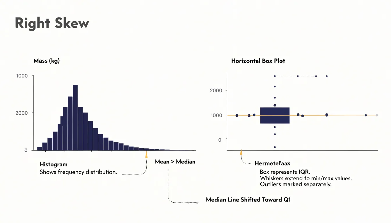
The box plot translates the same asymmetry through the median’s offset toward Q1 (for right skew) or Q3 (for left skew) alongside the corresponding extended whisker.
Comparing the two views side by side reinforces the connection between them. The quartiles marked by the box edges correspond to the regions where the histogram’s bars are densest, while the whiskers span the thinner tails. Seeing a long right tail on a histogram and an offset median with an extended upper whisker on a box plot describes the same underlying shape from two angles. Together, they let a reader confirm skewness visually and judge how strongly it shapes the data.
Box Plot
A parallel box plot arrangement places several box plots side by side along a shared axis, a layout that is particularly effective when a dataset contains dozens of categories that need to be compared at once. Each box occupies a narrow vertical strip, so even twenty or thirty groups can fit comfortably across a single chart. The viewer’s eye can scan horizontally from one group to the next, registering differences in medians, the spread of the interquartile ranges, and the reach of the whiskers without needing to consult a legend or switch between separate charts.
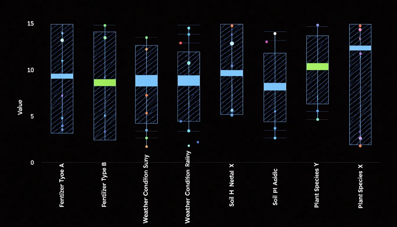
The compactness of the five-number summary is central to this strength. Because so little ink is required per group, many distributions can share one canvas. A histogram, by contrast, needs a full set of bars to describe each group, so combining even a handful of them quickly exhausts the available space. The box plot’s economy of marks keeps the display readable as the number of categories grows.
The side-by-side arrangement also makes variance easy to assess. Groups with tall boxes visibly signal greater spread in their middle fifty percent of values, whisker length communicates the reach of the tails, and stray points reveal outliers. Medians line up along a common baseline, allowing quick judgments about which categories sit higher or lower and how much the medians differ from one another. Analysts can therefore spot shifts in central tendency and changes in dispersion simultaneously, making parallel box plots a practical default for exploratory comparison across many groups.
Histogram
Sample size plays a central role in determining how much detail a histogram can reveal and how trustworthy the picture it presents will be. When a dataset contains thousands of observations, the values spread across the bins in a way that produces a smooth, continuous-looking distribution. Each bin collects enough observations for its height to reflect a genuine pattern in the data rather than random fluctuation, and the overall shape becomes a reliable summary of the underlying distribution.
Small sample sizes behave quite differently. With only a few dozen observations, many bins end up empty or nearly empty, so the histogram develops visible gaps and jagged peaks that have little to do with the true shape of the data. A bin that happens to catch two or three values can appear disproportionately tall, while neighboring bins may show almost nothing. These gaps and spikes can suggest trends that are not actually present, such as apparent clusters or missing regions in the data, when in reality they simply reflect the limited number of observations available.
This effect is especially pronounced when the number of bins is held constant across samples of different sizes. A fine-grained binning scheme that works well for a large dataset will fragment a small one into a sparse and erratic display. Analysts working with limited data often reduce the number of bins to compensate, which smooths out some of the noise at the cost of losing granularity. Recognizing this trade-off helps readers interpret a histogram honestly, understanding that smoothness signals sufficient data while gaps and irregular peaks may simply reflect a small sample rather than a meaningful feature of the underlying population.
Histogram
Because every part of the data range receives visible representation in a histogram, features that summary statistics compress away remain on display. A mean and standard deviation can describe a symmetric, single-peaked dataset well, yet the same two numbers can arise from wildly different underlying distributions. When a second peak, an isolated cluster, or an empty stretch of values exists, the histogram renders it as a visible feature rather than a fact buried in the numbers.
Bimodal peaks are a common example. A combined dataset of measurements from two distinct processes often shows two humps, each corresponding to one source. The overall average may land in the sparse valley between them, describing no actual observation. The histogram makes this separation obvious and invites the analyst to split the data and investigate each mode on its own terms.
Gaps and unexpected clusters appear in the same way. A clean break in the bars can signal a threshold, a change in instrumentation, or a subgroup with different behavior. A small detached cluster at one edge may point to outliers that belong to a separate population entirely. In each case the histogram exposes structure that averages, medians, and ranges smooth over.
This capacity to reveal hidden patterns makes the histogram a natural first step in exploratory analysis. Before choosing models or computing test statistics, plotting the distribution shows whether the data is unimodal, skewed, or segmented. Those observations guide every later decision, and they emerge directly from the shape the histogram draws.
Both Charts
Spread is the dimension of a dataset that describes how observations fan out around the middle, and both charts give that dimension a visible shape. A histogram’s silhouette reveals density directly: where the data clusters, the bars rise; where observations thin out, the bars shrink. You can see how abruptly frequencies fall away toward the extremes. Range emerges as the width of the occupied bins, and overall variance is visible in how widely the mass of bars is dispersed rather than concentrated in a narrow band.
A box plot condenses the same underlying spread into exact landmarks. Because the quartiles, 1.5×IQR whisker ends, and outlier positions translate directly into measurable quantities rather than visual impressions, the box plot is ideal for quoting and comparing spread across groups.
Used together, the two charts cover the analysis from complementary angles. The histogram shows the texture of the distribution, while the box plot supplies the precise bounds against which spread, variance, and range can be compared.
Both Charts
Applying both chart types to real-world datasets makes their complementary strengths concrete:
- Regional housing prices: A histogram of sale prices reveals whether prices cluster tightly around a central value or spread into a long right tail caused by a handful of luxury properties. The same data rendered as a box plot instantly surfaces the median sale price, the IQR, and any outlier mansions sitting far above the upper whisker. Analysts comparing several neighborhoods can place box plots side by side to rank median prices and compare spread at a glance, while a histogram remains the better tool for understanding the shape of a single neighborhood’s price curve.
- Customer wait times: A histogram of wait times at a service center shows whether most customers are served quickly with a few long delays, or whether waits are broadly uniform. Because wait time data is often skewed, the box plot becomes valuable for flagging extreme delays as outliers and for comparing performance across branches, shifts, or days of the week. Operations teams can monitor a dashboard of box plots to spot a branch whose median wait is drifting upward, then drill into a histogram to understand the underlying pattern.
- Exam scores: A histogram of scores shows the distribution of student performance, revealing whether the class clusters around a passing grade or splits into distinct groups. Box plots comparing scores across classrooms or cohorts make it easy to compare medians, spot unusually low or high performers, and judge the consistency of results.
Together, these walkthroughs show that histograms excel at revealing distribution shape and modality, while box plots excel at summarizing and comparing groups with compact statistics. Using them in tandem gives analysts a fuller picture of any dataset than either chart provides alone.
Both Charts
Common mistakes with box plots and histograms tend to cluster around a few recurring sources of confusion. One frequent error involves misinterpreting the areas inside a box plot. Although the box length represents the IQR, readers often treat the visual area or width of the box as a direct measure of spread or frequency. The width of a box plot carries no data meaning in most software defaults, so a wide or narrow box says nothing about sample size or density. The whiskers introduce a related problem: because points beyond 1.5×IQR are flagged as outliers, readers may treat them as errors even when they belong to a legitimate heavy-tailed distribution.
With histograms, bin configuration is the top pitfall. Because both bin width and starting position affect whether the chart hides real structure or creates noisy spikes, two analysts can plot the same data and reach different conclusions about its shape.
A broader misjudgment concerns dataset shape. Readers may infer skewness or modality from a box plot that only reports five summary statistics, or they may read a histogram’s apparent peaks as real clusters when they reflect binning artifacts. Small samples amplify all of these problems. Overlapping groups, unequal sample sizes, and logarithmic axes add further opportunities for misreading. Careful annotation of bins, axis scales, and summary definitions helps readers avoid these traps.
Both Charts
Pairing a histogram with a rug plot or overlaying a box plot turns two complementary views of a dataset into a single, information-rich display. A rug plot adds a thin strip of tick marks along the histogram’s axis—one per observation—so individual data points remain visible even as the histogram summarizes them into bars. This combination is especially helpful for spotting gaps, isolated outliers, or ties that binned counts can obscure. Readers can see both the overall distribution and the exact locations of unusual values without consulting a second chart.
Overlaying a box plot on a histogram goes a step further by placing summary statistics directly on top of the frequency view. The box, median line, and whiskers mark the quartiles, central tendency, and spread of the bulk of the data, while the histogram behind them shows the full shape of the distribution. This makes it easy to relate a numeric summary, such as the IQR, to the visual pattern of bars around it. When the median sits off-center within the box or the whiskers differ in length, the overlay makes the underlying skew or heavy tail immediately apparent.
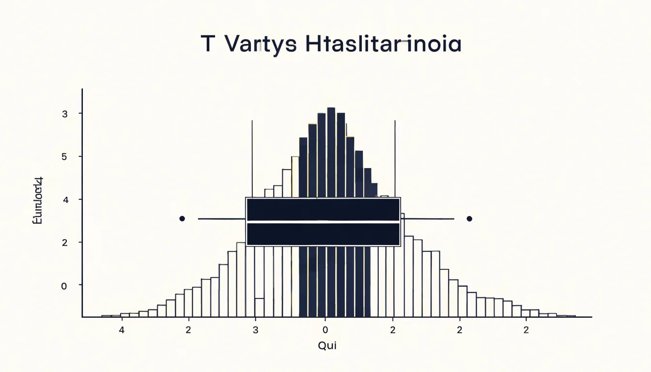
These combined displays serve well in reports, dashboards, and exploratory analysis, where a single panel must answer several questions at once: What is the typical value? How spread out is the data? Are there outliers? What is the overall shape? By capturing detailed frequency and summary statistics together, the paired chart reduces the need for back-and-forth between separate graphics.
Overview
When you are deciding between a histogram and a box plot, a short checklist grounded in three practical considerations will usually settle the question quickly:
- Dataset size: Histograms work well when you have a moderate to large number of observations, since the shape only becomes reliable once enough points fall into each bin. With very small samples, a histogram can look lumpy and misleading, while a box plot remains readable because it summarizes the data through quartiles and extremes without needing many bins.
- Audience’s statistical literacy: Box plots compress information into a compact form built around the median, IQR, whiskers, and outliers. Readers comfortable with these conventions can extract a great deal at a glance, but audiences unfamiliar with them may misread the box or wonder what the whiskers represent. Histograms tend to be more immediately intuitive, since tall bars plainly show where values cluster.
- Detail vs. summary comparison: When the shape of a single distribution matters—including skew, gaps, and multiple peaks—a histogram reveals those features directly. When you need to compare several groups side by side, box plots line up neatly and keep the visual field uncluttered, whereas stacked histograms can become crowded and hard to parse.
Run through these three questions before you build the chart: how many observations do you have, who will read the result, and are you showing the texture of one distribution or comparing summaries across groups? The answers usually point to a clear choice.
Frequently Asked Questions
What is the difference between a histogram and a box plot?
A histogram divides continuous data into bins and uses bar heights to show frequency, while a box plot summarizes a dataset using the five-number summary. Histograms reveal distribution shape, while box plots are compact for showing center, spread, skew, and outliers.
How do I choose the right bin width for a histogram?
Bin width is critical: too few bins can oversimplify the distribution and hide details, while too many can produce a noisy plot. Analysts often experiment with different widths or use Sturges’ formula or the Freedman-Diaconis rule as starting points.
What do the whiskers and points beyond them mean in a box plot?
Whiskers are often drawn to the most extreme observations within 1.5 times the IQR from the quartiles, and points beyond the whiskers are plotted individually as outliers. The 1.5×IQR rule is a descriptive heuristic, not a statistical test.
How can I tell if data is right-skewed or left-skewed from a box plot?
If the median is closer to Q1, the data are right-skewed; if the median is closer to Q3, the data are left-skewed. A longer upper whisker signals right skew, and a longer lower whisker signals left skew.
How does sample size affect a histogram?
With thousands of observations, a histogram can produce a smooth, reliable picture, but with only a few dozen observations, many bins may be empty or nearly empty and create gaps and jagged peaks. Analysts working with limited data often reduce the number of bins to compensate, which smooths noise at the cost of granularity.
When should I use a histogram instead of a box plot?
Use a histogram when the shape of a single distribution matters, including skew, gaps, and multiple peaks, and use box plots when comparing several groups side by side. Dataset size and the audience’s statistical literacy are also practical considerations.
Tony Astor
Tony writes about data visualization and the tools people use to build charts and dashboards. More about Data Illustrator