Hexbin Map: Equal-Sized Tiles for Geographic Data
 By Tony Astor ·

Hexbin Map
A hexbin map is a visualization that divides geographic space into a uniform grid of equal-sized hexagonal cells, aggregating data within each cell and shading it by count or value. Because every hexagon carries equal visual weight, dense areas stand out while sparse regions recede, eliminating the area bias of choropleth maps.
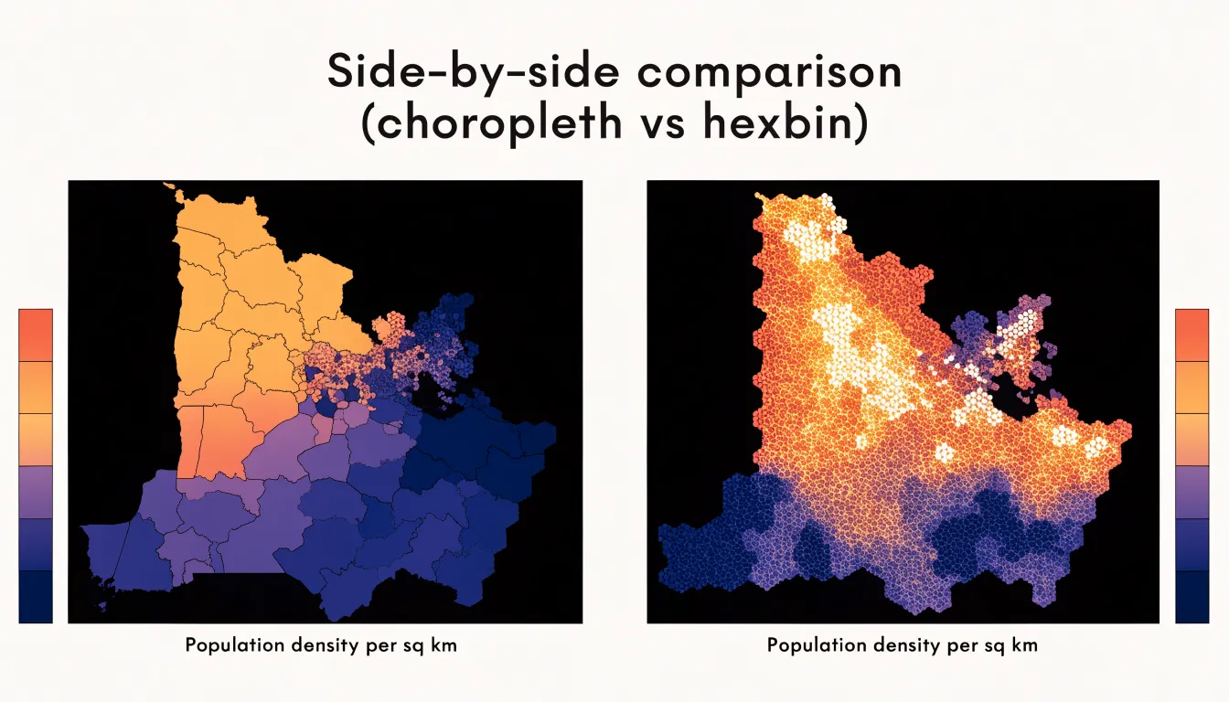
Table of Contents
Hexbin Map
Traditional choropleth maps assign a single color value to an entire administrative region, whether that region is a sprawling rural county or a compact city district. Because the visual weight of each shape is proportional to its geographic area, vast territories with few residents dominate the viewer’s attention simply because they occupy more pixels on the page. A sparsely populated county covering thousands of square miles draws the eye far more than a dense urban core squeezed into a handful of square kilometers, even when the urban area contains many times the population. This mismatch between visual prominence and the number of people represented is the central distortion of the choropleth approach.
The problem compounds when averages are calculated across large regions. A single value summarizing a whole county flattens internal variation, hiding pockets of high density inside otherwise empty land and masking neighborhood-level differences within cities. Readers come away with an impression shaped by land area rather than by population, and that impression can invert the actual story in the data. A metropolitan region with millions of residents may appear as a tiny speck of color surrounded by broad expanses of countryside, leading viewers to underestimate its importance.
Hexbin maps address this by tessellating space into uniform hexagonal cells and aggregating data within each cell. Because every bin covers a comparable area and receives equal visual weight, no region gains influence merely from its size. Dense clusters of population light up as concentrations of color, while empty expanses remain visually quiet. The hexagonal shape also reduces the edge and orientation artifacts that square grids introduce, producing smoother gradients across neighboring cells. For questions about where people actually live and how density varies across a landscape, the hexbin layout gives a faithful picture in which the viewer’s attention tracks the distribution of the underlying phenomenon rather than the arbitrary geometry of political boundaries.
Hexbin Map
At the heart of the hexbin map lies a principle borrowed from geometry and cartography alike: spatial tessellation. A geographic area is partitioned into a grid of adjoining cells that fit together without gaps or overlaps, covering the territory completely. Although squares and triangles can serve the same purpose, what matters is the deliberate division of continuous space into discrete, manageable units. Each tile becomes a container for a fixed portion of the map, gathering and summarizing every record within its boundaries as a count, an average, or another statistic. This division transforms a chaotic cloud of scattered points into a uniform, structured surface of visual marks.
The choice of equal-sized tiles carries real consequences for visual honesty. Human perception is poorly equipped to judge density when marks differ in size. When every hexagon occupies the exact same screen area regardless of where it sits, the reader’s attention goes straight to the visual channels that actually encode the data values: color, height, or shading.
Uniform tiles also neutralize the distortions introduced by map projections, where areas near the poles or along the edges stretch and compress relative to the center. In a hexbin grid, a tile near the equator and a tile near the pole claim equal visual real estate. A high value stands out for its magnitude rather than for the physical space it happens to occupy, keeping comparisons fair across the entire map.
Hexbin Map
When selecting a grid for aggregating spatial data, choosing hexagons over squares carries significant implications for the accuracy and interpretability of the resulting map:
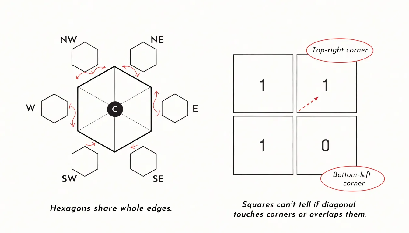
- Superior edge-sharing: Each hexagon shares an edge with six neighbors, whereas a square shares edges with only four. This uniform adjacency eliminates the corner-touching ambiguity inherent in square grids, where diagonal neighbors meet at a single point. The result is a more connected representation of spatial relationships with fewer orientation artifacts.
- Reduced quantization error: Assigning continuous data points to discrete grid cells inevitably introduces error. Because hexagons approximate a circle more closely than squares do, they minimize the maximum distance from any point in the cell to the cell centroid. This leads to a lower average quantization error than in squares, where points near corners sit significantly farther from the center, allowing hexagonal binning to preserve sparse or clustered distributions more faithfully.
- Isotropic centroid distances: In a square grid, the distance between centroids of adjacent cells is uniform along the axes but larger for diagonal neighbors, creating directional bias. Hexagons have centroids that are equidistant from all six neighboring centroids, providing a uniform metric space. This isotropy ensures that analyses such as distance-based clustering or spatial autocorrelation are not distorted by grid orientation, which is especially beneficial when modeling phenomena that spread uniformly in all directions.
Hexbin Map
Because population, sales, incidents, and sensor readings rarely distribute themselves in proportion to land area, the unequal footprint of administrative territories can severely skew analysis. In a conventional choropleth, a single sprawling province or desert district with a moderately high value can pull the eye away from dozens of compact urban municipalities whose combined activity dwarfs it.
Hexagonal binning equalizes these footprints by construction. When data are aggregated into uniform cells and colored by their summarized values, a dense cluster of high-value bins reads as a prominent cluster regardless of whether those bins sit inside a vast rural jurisdiction or a tiny city. Furthermore, because every bin shares the same six-neighbor geometry, readers can compare adjacent cells directly across the map without fighting the strong diagonal artifacts of square grids. Removing the area advantage of large territories lets the spatial pattern of the data itself drive interpretation.
Hexbin Map
A hexbin map turns raw latitude and longitude coordinates into a structured grid through the binning process. Because the grid covers the coordinate plane without gaps or overlaps, the assignment rule stays unambiguous: each point is assigned to the single hexagon whose boundaries contain its coordinates (or, equivalently, whose center is nearest to it). During this step, the individual records are tallied, averaged, or summed per cell, producing a table of hexagon identifiers paired with aggregate values.
This hexagonal geometry has practical benefits for the binning algorithm. Because the distance from one cell center to any adjacent cell center is constant, the aggregation neighborhood remains uniform in every direction. The resulting tiles avoid the directional bias that appears when rectangular grids measured in degrees of latitude and longitude distort toward the poles, and they follow the curved silhouette of natural data distributions more closely than squares.
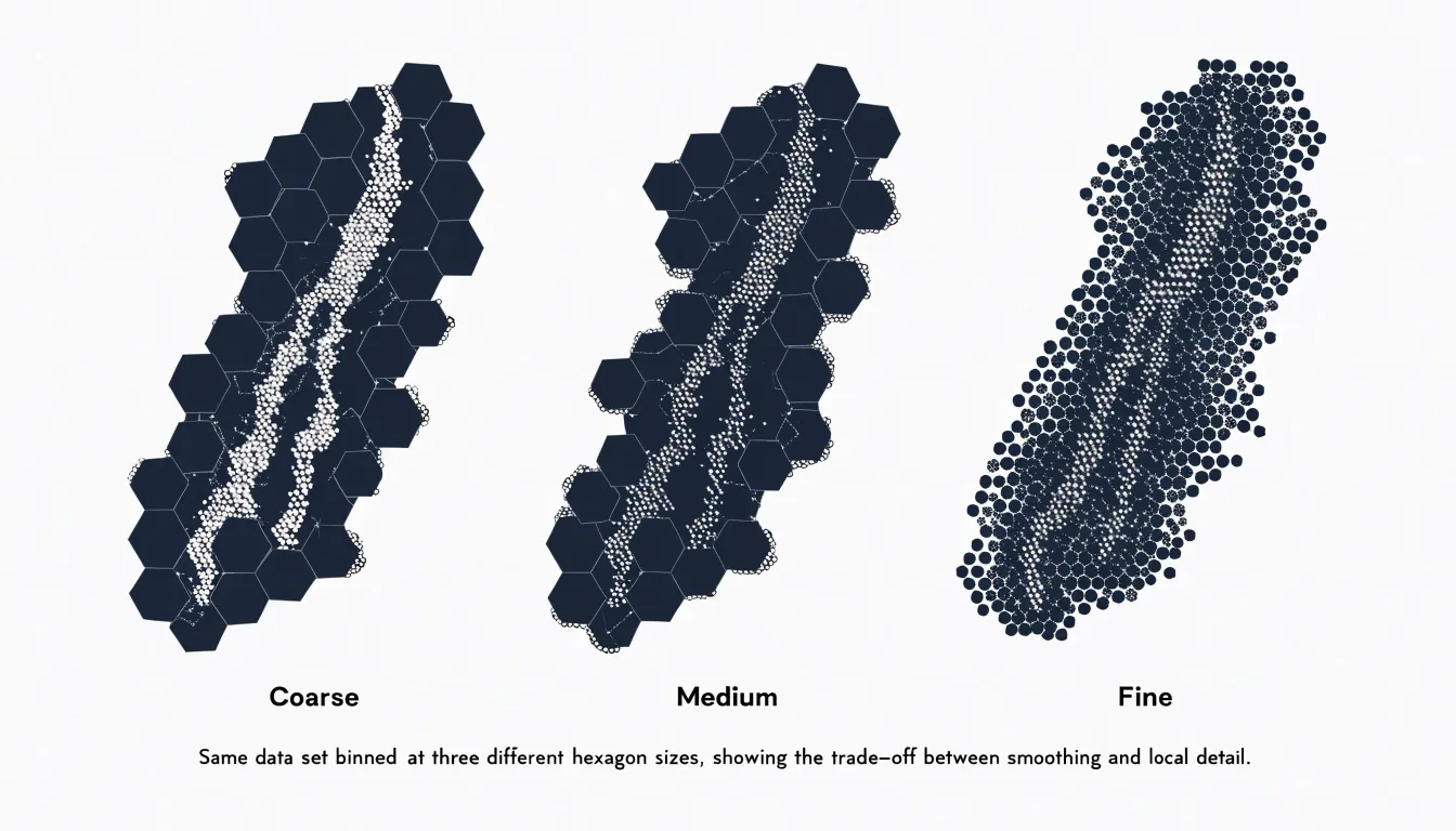
The analyst controls the resolution of this process by setting the cell size, which determines how many points each hexagon receives. Smaller hexagons preserve local variation and reveal fine-grained structure, while larger hexagons smooth out noise and emphasize regional trends. This makes hexbin mapping especially useful for dense datasets where plotting every point would cause heavy overplotting, condensing thousands of observations into a readable surface.
Hexbin Map
Sequential color palettes form the visual backbone of a hexbin map’s ability to communicate density. A sequential palette moves through ordered steps of lightness and saturation, typically from a pale, low-intensity hue for tiles with few points to a deep, saturated hue for dense tiles. Because the human eye perceives changes in lightness and saturation with reasonable accuracy, this ordered ramp lets viewers compare counts quickly across the map without looking up every region in a legend.
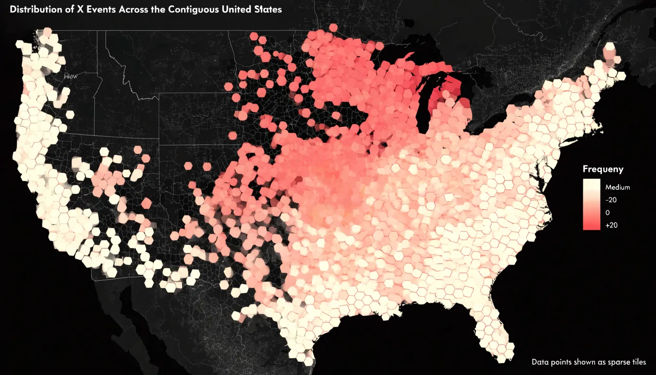
Opacity variations add a second layer of refinement. Applying partial transparency to lighter tiles lets the underlying basemap show through, providing geographic context for sparse areas while keeping them visually distinct. Rendering dense tiles at full opacity saturates the color and draws attention to the concentrations that matter most. Tuning opacity alongside the palette keeps the visual hierarchy coherent: low-count regions recede gently into the background, and high-count regions advance toward the viewer.
When the palette and opacity are aligned in the same direction, the map reads as a continuous field of intensity rather than a patchwork of disconnected shapes. Smooth transitions across neighboring tiles reveal density gradients, hotspots stand out as dark clusters, and transitional zones appear as intermediate tones that invite closer inspection.
Hexbin Map
When a conventional choropleth renders a sprawling rural district at twenty times the screen area of a dense urban core, cartograms and equal-area hex grids offer two complementary ways to restore visual parity.
Cartograms give every location an equal voice by resizing each administrative region in proportion to a chosen variable, such as population or event counts, rather than its geographic footprint. A small municipality with a large population swells to reflect its demographic weight, while a vast, lightly inhabited territory contracts. Equal-area hex grids take a different route: instead of warping existing political borders, they impose a uniform lattice of identical hexagons over the study area. Small entities are never squeezed into illegibility, and large ones cannot crowd out their neighbors. Both approaches allow analysts and audiences to compare regions on a level footing, confident that visual emphasis tracks the phenomenon under study rather than sheer acreage.
Hexbin Map
Beyond varying in size, administrative boundaries such as counties, states, and zip codes are political or bureaucratic divisions that rarely align with natural phenomena. A county with a large rural expanse might report a low overall average, masking a concentrated cluster of high values in one corner, or an arbitrary border might slice a single cluster in two.
By imposing a grid that is independent of political jurisdictions, hexbin maps allow continuous spatial distributions to emerge organically from the data. Gradients and hotspots can be tracked seamlessly across municipal or state lines. This unfiltered view is particularly valuable in fields like epidemiology, where disease outbreaks spread across regions regardless of jurisdiction, and in urban planning, where commuting patterns and land use routinely transcend city limits.
Hexbin Map
The choice of grid resolution is the single most consequential decision when constructing a hexbin map. Because cell size determines how much information is combined into a single mark, a resolution that is too coarse collapses distinct clusters into broad, featureless blobs, masking local variation. Conversely, a resolution that is too fine scatters observations across so many small cells that the map loses its smoothing effect and begins to resemble a dot map with irregular gaps. Finding the right balance depends on the density of the input data, the geographic extent of the study area, and the questions the map is meant to answer.
A practical starting point is to evaluate the average number of points expected per cell. When most occupied cells contain a reasonable count, the color ramp communicates meaningful differences in density rather than random noise. Analysts often test several candidate resolutions side by side to check whether known features—such as urban cores, transportation corridors, and natural boundaries—stay legible. If these features dissolve into uniform shading, the cells are too large; if they fragment into isolated specks, the cells are too small. Interactive tools that adjust resolution in real time are also helpful, as the ideal scale often depends on the zoom level.
For operational decisions like identifying local hotspots or allocating field resources, preserving fine granularity to distinguish neighboring areas is essential, even at the cost of some visual smoothness. For high-level overviews, a coarser grid usually works better to emphasize broad patterns without overwhelming the reader. Documenting the chosen resolution and the reasoning behind it helps audiences interpret the map correctly and supports reproducibility when the analysis is revisited.
Hexbin Map
Preparing coordinates for grid placement is the foundational step in building a hexbin map, and the quality of this preparation determines how faithfully the final visualization represents the underlying data. Raw coordinate data rarely arrives ready for binning:
- Clean and validate records: Remove entries with missing latitude or longitude values, parse coordinates stored as text strings into numeric values, and flag anomalies—such as points landing in the ocean when the dataset describes land-based events. Deduplicate the data as well, since repeated points inflate counts within individual hexagons and distort the density pattern.
- Convert map projections: Geographic coordinates are typically stored in degrees of latitude and longitude on a spherical or ellipsoidal model, whereas a hexbin layout operates on a flat plane. Reproject the data into a suitable planar coordinate reference system (CRS) appropriate to the study region. Because hexagon size and placement are computed in planar units, skipping this step introduces visible skew in how points cluster.
- Normalize and assign coordinates: Map the projected points onto the uniform coordinate plane by normalizing them to the grid’s extent and assigning each record to its containing hexagon. Handle boundary cases—where a point sits directly on a hexagon edge—deterministically so that point assignment remains consistent across runs.
Hexbin Map
Overplotting isn’t limited to geographic maps; when any two-dimensional scatter plot contains thousands or millions of data points, overlapping markers collapse into solid blocks of ink that hide the true distribution. Hexagonal binning solves this for standard x-y charts as well. By overlaying a tessellated hexagonal grid onto the Cartesian coordinate space of the scatter plot, the chart tallies the points falling into each x-y bin and encodes that count using a sequential color ramp.
The resulting density plot preserves the overall shape of the data cloud while making local concentrations inside saturated regions legible. Analysts can compare clusters across categories and spot internal gradients that a traditional scatter plot would flatten into a uniform mass. Because each cell summarizes many records, the visualization scales gracefully to massive datasets while keeping the visual weight of the chart stable.
Hexbin Map
Electoral maps built on geographic boundaries suffer acutely from the area-size distortion of standard choropleths. When administrative units are filled with color proportional to vote share, sparsely populated rural districts dominate the page while dense cities containing millions of voters shrink to barely visible slivers. Such a map reports territorial winners accurately but communicates political magnitude poorly.
In electoral cartography, a hexbin map replaces irregular voting districts with a uniform grid where each hexagon represents an equal-population bin or a standardized reporting unit. A densely settled urban area therefore occupies many hexagons, while a sprawling rural county occupies only as many as its population warrants. Positioned to approximate real-world geography while discarding arbitrary polygon borders, these hexagons draw the viewer’s eye in proportion to voters rather than acreage. Analysts and general audiences alike can then compare turnout, victory margins, and vote swing using a consistent visual currency across the entire political landscape.
Hexbin Map
Wildlife biologists and environmental scientists rely on high-volume data streams to study ecosystem dynamics: GPS collars on migratory animals emit frequent location pings, remote sensors log temperature, humidity, and air quality, and field observers record species sightings. Aggregating these millions of records into a hexbin grid turns an unreadable cloud of pings into a clear surface of ecological activity, while the isotropic nature of the hexagonal grid ensures that researchers can track movement—such as a herd of caribou or a population of sea turtles—without directional distortion.
Furthermore, the uniform grid acts as a common spatial framework for combining disparate data sources. Analysts can overlay animal GPS pings with environmental sensor logs in the same cells to see how wildlife movement aligns with habitat conditions; a corridor where animal activity clusters alongside rising temperatures immediately stands out as adjoining high-value bins.
Generating hexbin maps across successive seasons or years adds a temporal dimension. By comparing cell densities over time, researchers can detect shifts in migration routes, range expansion or contraction, and emerging hotspots. Cells that gain or lose density reveal habitat pressure, climate stress, or conservation success, supporting adaptive management as environmental conditions evolve.
Hexbin Map
In commercial operations, mapping sales leads, delivery requests, or user sign-ups onto a hexbin grid shows organizations where demand concentrates across their territories:
- Retail and field operations: Aggregating customer addresses reveals clusters of activity that guide store or pop-up placement. Field operations teams use the same view to spot where service requests pile up and where coverage is thin, allowing them to route staff efficiently and schedule visits around genuine demand.
- Sales and logistics: Plotting multi-channel sales leads into a shared hexbin layer produces a unified density surface for territory planning and quota allocation. Similarly, mapping delivery requests highlights high-volume corridors that justify dedicated shipping routes or new distribution centers.
- Market expansion: When launching in new markets, binning user sign-up locations shows which neighborhoods generate organic traction and which remain underserved, informing localized marketing spend and partnership opportunities. By tuning grid resolution, planners can seamlessly transition from regional overviews down to street-level hotspots.
Hexbin Map
Hexbin maps become far more useful when embedded in a dynamic dashboard—such as in Tableau, Power BI, or a custom D3.js build—rather than viewed as a static image.
Interactive hover states are the first step: moving a cursor over a hexagon should trigger a compact tooltip revealing the bin’s aggregate value, its record count, and secondary measures like average revenue or conversion rate, accompanied by subtle cell highlighting or a change in border weight. Cross-filtering extends this interactivity across the dashboard. Clicking a hexagon can filter adjacent charts, tables, and key performance indicators in real time, letting analysts move from a broad spatial overview to a focused segment on the same page. Smooth zooming complements this workflow by interpolating between zoom levels and loading finer-grained bins as the view narrows, allowing local detail to emerge naturally without abrupt redraws.
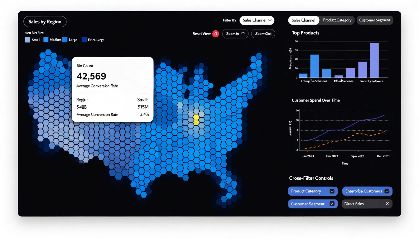
Implementing these behaviors requires attention to performance and visual stability. Aggregations should be precomputed or cached where possible, tooltips must render without lag, and filter events should debounce so rapid interactions do not overwhelm the rendering layer. Finally, color scales and legends should update predictably across zoom and filter states, turning the hexbin map from a decorative summary into an active instrument for exploration.
Frequently Asked Questions
What is a hexbin map and what problem does it solve?
A hexbin map tessellates space into uniform hexagonal cells and aggregates data within each cell. This gives every bin equal visual weight, so dense clusters are not overshadowed by large geographic regions as they can be in traditional choropleth maps.
Why use hexagons instead of squares in a hexbin map?
Hexagons share edges with six neighbors, avoiding the corner-touching ambiguity of square grids. They also reduce quantization error and provide isotropic centroid distances, which helps avoid directional bias.
How do I choose the right grid resolution for a hexbin map?
Grid resolution is the most consequential choice and depends on the input density, geographic extent, and questions the map should answer. A coarse grid can collapse distinct clusters, while a grid that is too fine begins to resemble a dot map with irregular gaps; testing several resolutions helps keep known features legible.
How should color and opacity be used in a hexbin map?
A sequential palette should move through ordered steps of lightness and saturation, typically from pale for low-count tiles to deep for dense tiles. Partial transparency can let the basemap show through in sparse areas, while dense tiles at full opacity draw attention to concentrations.
What data preparation is needed before binning points in a hexbin map?
Clean and validate records by removing missing coordinates, parsing text coordinates into numbers, flagging anomalies, and deduplicating repeated points. Then convert map projections into a suitable planar coordinate reference system and assign normalized coordinates to hexagons, handling boundary cases deterministically.
How can a hexbin map be made interactive in a dashboard?
In a dashboard, hover states can show tooltips with the bin’s aggregate value, record count, and secondary measures, while cross-filtering lets a clicked hexagon update other charts and indicators. Zooming can load finer-grained bins, and aggregations should be precomputed or cached, tooltips rendered without lag, and filter events debounced.
Tony Astor
Tony writes about data visualization and the tools people use to build charts and dashboards. More about Data Illustrator