Heatmap vs Choropleth Map: What's the Difference?
 By Tony Astor ·
Heatmap vs Choropleth Map
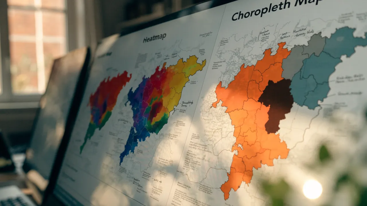
A heatmap visualizes point data as a continuous density surface using kernel density estimation, revealing hotspots and gradual transitions without fixed boundaries. A choropleth map shades predefined regions, such as counties or census tracts, with aggregated values. Use heatmaps for raw point data and choropleths for pre-aggregated regional statistics.
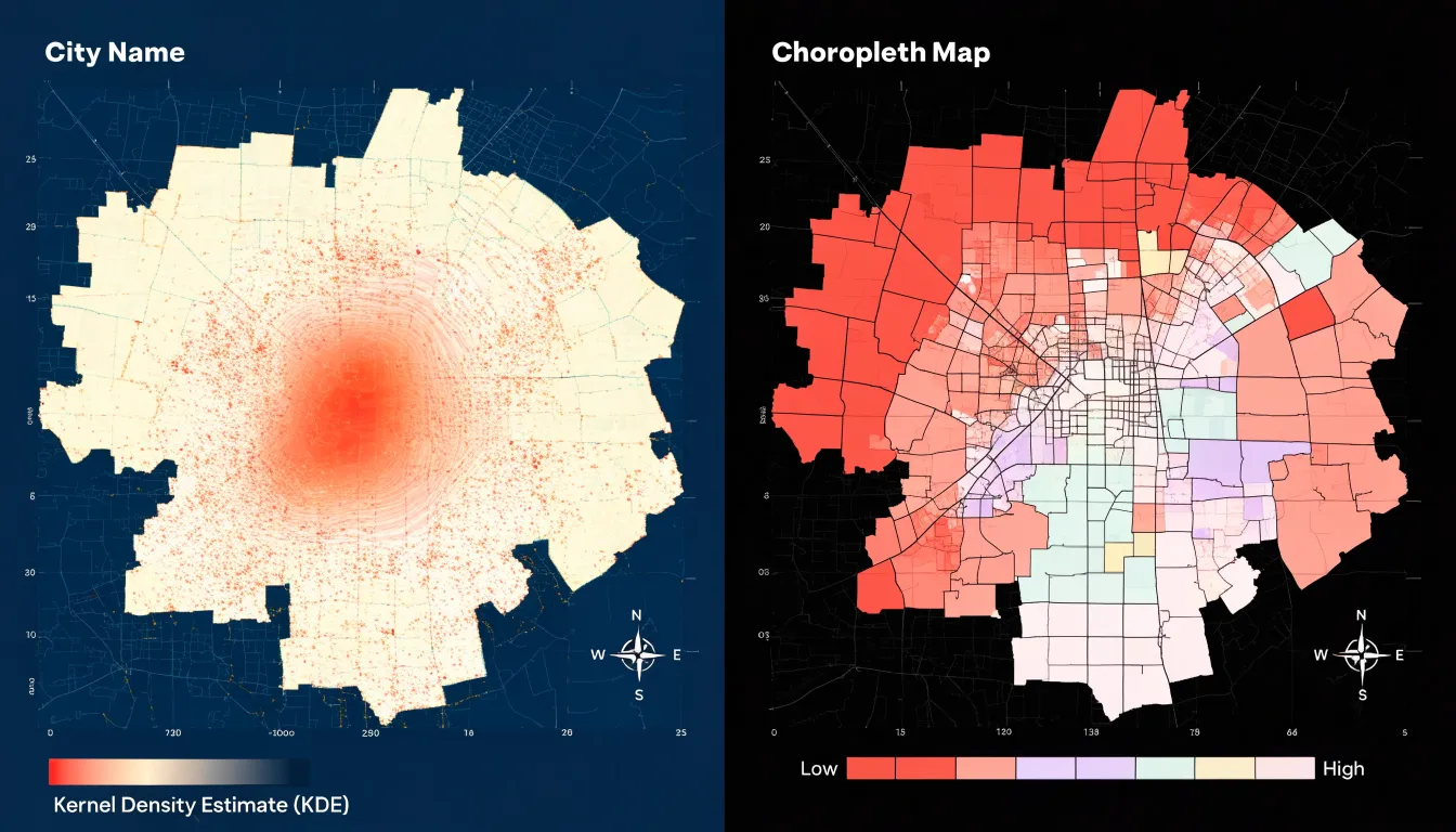
Table of Contents
Heatmap
A heatmap visualizes the concentration and intensity of a phenomenon across open space, treating geography as a continuous surface rather than a collection of bounded shapes. Points of activity—such as incidents, customers, or observations—are plotted individually, and a kernel density estimation algorithm calculates a smooth surface of intensity around them. Each point contributes a small field of influence that fades with distance according to a chosen kernel function and bandwidth, and where these fields overlap, density values accumulate. The result is a gradient that reveals hotspots, clusters, and gradual transitions, showing where activity concentrates and how quickly it thins out as one moves away.
Because the computation relies on the positions of the underlying data rather than on predefined administrative borders, a heatmap can follow patterns wherever they occur. A cluster straddling a city limit, a corridor of activity crossing several districts, or a diffuse spread that no polygon neatly captures all appear naturally in the rendered surface. The boundaries visible on the map emerge from the data itself, and analysts can adjust the bandwidth to emphasize broad regional trends or finer local detail. This flexibility makes heatmaps well suited to exploratory analysis, where the goal is to detect structure before any decision is made about how space should be divided.
Interpretation requires care. The smooth surface is a modeled estimate rather than a count, so the values represent relative intensity rather than exact totals. Color choices and bandwidth settings strongly shape the visual impression, and large areas of sparse or absent data can be misread as meaningful low-density zones. Providing a legend, stating the bandwidth, and noting the sample size behind each point help readers interpret the map accurately.
Choropleth Map
A choropleth map divides a geographic area into fixed, predefined units—such as counties, states, census tracts, or countries—and shades each unit with a color that represents an aggregated value for that region. Because the boundaries are established independently of the data, the map maker begins with a ready-made set of polygons and joins summary statistics to them. For example, a choropleth of population density by county calculates one value per county, typically by summing or averaging the underlying records for all people or households within that boundary, and assigns that number to the entire polygon. A color scale, or fill scale, then maps each value range to a specific shade so readers can compare regions at a glance.
This aggregation step is central to how choropleths communicate. Individual data points such as addresses, survey responses, or sensor readings are folded into their containing unit, so the map displays regional totals, rates, or averages rather than the raw points. This produces a clean picture that highlights broad geographic patterns: clusters of high values, sharp transitions between neighboring units, and large areas of uniform color. Because every polygon is filled, even regions with very few underlying observations receive a visible fill, which keeps the map continuous and easy to scan.
The choice of unit shapes the map’s message. Counties, states, and countries vary enormously in size and population, so large rural units can dominate the visual field while small, densely populated units appear as tiny slivers. Designed carefully, choropleths turn aggregated values into a readable surface of shaded regions that supports quick regional comparison.
Core Design Differences
The core design differences between heatmaps and choropleth maps emerge most clearly in how each renders color across space. A heatmap produces continuous gradients, where color flows smoothly from one value to the next without interruption. The surface has no hard edges; instead, hue and intensity shift gradually as density changes, creating a soft, cloud-like diffusion across the canvas. This smooth transition allows the eye to follow subtle changes in magnitude, since each point blends into its neighbors and the overall image reads as a single continuous field.
A choropleth map works with a fundamentally different visual grammar. Each predefined region receives a single fill value that stops abruptly at the polygon’s edge. The result is a patchwork of rigid shapes with sharp boundaries between adjacent units and no intermediate blending along the border.
This contrast shapes what each map communicates about space:
- Continuous gradients (heatmaps) suggest that the underlying phenomenon varies smoothly and that boundaries are arbitrary overlays on a fluid reality. The smooth surface invites readings of flow, concentration, and gradual transition.
- Fixed area shading (choropleths) implies that the unit itself is the meaningful container of the value. The polygonal fill emphasizes categorical membership and regional comparison.
Designers choosing between the two are deciding whether the visual language should express seamless variation or discrete territorial assignment, a decision that shapes how viewers perceive the underlying geography.
Matching Data Types
Point coordinates and regional statistics follow different data structures and support different analytical goals. A dataset of raw latitude-longitude readings records individual events or observations at precise locations, such as a sensor reading, a customer address, a traffic incident, or an animal sighting. Each record carries its own position in space, and the collection of points builds meaning through density. A heatmap works directly from this structure, keeping the individual point as the underlying unit of analysis to reveal patterns of concentration without any prior grouping.
Regional statistics assign one value to an existing administrative or statistical area, such as a postal code, census tract, county, or district. The value often arrives as a standardized metric: a rate, a ratio, a percentage, or an index adjusted for area or population. A choropleth map is built for this structure, treating the whole region as a single analytical unit. Because the boundaries are fixed in advance, interpretation depends on the accuracy and fairness of the statistical aggregation behind each polygon.
Matching the data to the method keeps the visualization honest. Feeding point coordinates into a choropleth requires arbitrary grouping and can distort the underlying locations, while forcing pre-aggregated regional statistics into a heatmap produces a misleading surface unsupported by individual observations.
How Heatmaps Work
A heatmap begins with discrete data points, each carrying a location and often a weight or intensity value. To turn these isolated marks into a continuous surface, the mapping process applies a density estimation technique built around Gaussian kernels. Each point is treated as the center of a small bell-shaped curve whose value falls off gradually as distance from the point increases. The kernel’s width, or bandwidth, determines how far a single point’s influence spreads. A narrow bandwidth keeps each point’s contribution tight and localized, while a wider bandwidth lets it radiate over a larger area, blending more readily with neighboring points.
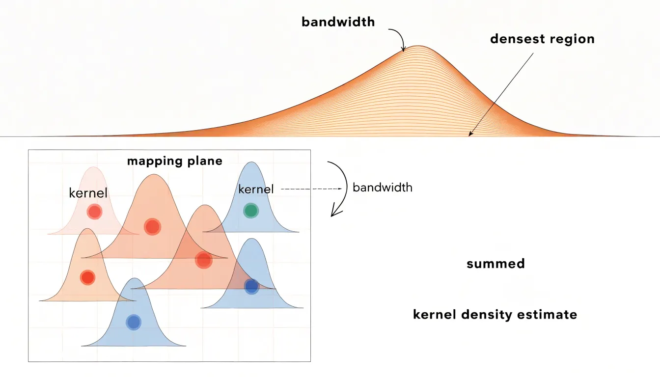
Once a kernel is assigned to every point, the values from overlapping kernels are summed at each location on the map surface. Where many points cluster together, their individual curves stack and produce elevated values; where points are sparse, the summed value stays low. Radius thresholds refine this step by defining a cutoff distance beyond which a point’s contribution is treated as zero. This limit keeps computation manageable and prevents distant points from subtly inflating values in areas where no real activity exists.
The summed kernel values are then normalized, typically by dividing by the total weighted count, so that the resulting surface reflects relative intensity rather than raw totals. That surface is finally rendered through a color gradient, with high-value zones appearing as warm or saturated hotspots and low-value zones fading into cooler or lighter tones. Because the kernel bandwidth and radius threshold shape the final picture considerably, analysts tune these parameters to match the scale of the patterns they want to reveal.
How Choropleths Work
Building a choropleth map begins with aggregating raw observations into a representative value for each region, typically an average, a rate, or a ratio, often normalized per capita or as a percentage. Once every boundary holds a value, those values are sorted and divided into classes. This classification step determines how much visual variation the reader will perceive, and different methods produce noticeably different maps from the same dataset:
- Equal-interval classification splits the range between the minimum and maximum into evenly sized bins, which suits data spread uniformly across space. However, it can collapse most regions into a single shade when one extreme outlier stretches the range.
- Quantile classification places an equal number of regions into each class, which emphasizes relative ranking and works well when values cluster at one end of the distribution. Its tradeoff is that it can exaggerate small differences among similar values.
- Natural breaks (Jenks) look for gaps in the data and place class boundaries where values jump, preserving clusters that exist in the underlying numbers.
After classification, each interval receives a color. Sequential palettes move from light to dark in a single hue or a narrow family of hues, which fits ordered data such as population density or median income. Diverging palettes place two contrasting hues at the extremes with a neutral light tone in the middle, which suits values measured against a meaningful midpoint, such as change relative to a national average or a positive-versus-negative balance.
Color Schemes
Color scheme selection differs between the two map types because one renders continuous density and the other represents discrete categories.
Heatmaps benefit from thermal gradients that mimic natural heat—such as yellow to red or blue to red—or single-hue and multi-hue sequential palettes. These continuous gradients allow viewers to perceive subtle variations in intensity. Rainbow palettes, while visually striking, introduce perceptual distortions and are generally discouraged for precise data interpretation.
Choropleth maps require distinct color scales with clear steps to differentiate categories. Using a continuous gradient for choropleth data can mislead viewers into thinking values change smoothly across boundaries, when in fact each region is a uniform category. Instead, a stepped color ramp with a limited number of classes ensures that each color represents a specific range of values. Beyond sequential and diverging palettes, choropleths can also use qualitative palettes when displaying purely categorical data.
Boundary and Distortion Pitfalls
Because choropleth maps rely on predefined geographic boundaries, they are vulnerable to a subtle but powerful distortion known as the Modifiable Areal Unit Problem (MAUP). MAUP occurs because the results of spatial analysis can change significantly when the boundaries of the units used for aggregation are modified, even if the underlying data remain the same. For example, a city’s census tracts can be drawn in many different ways, each yielding a different pattern of poverty or disease prevalence. The map user sees a clean, authoritative picture, but that picture is contingent on arbitrary decisions about where lines are drawn.
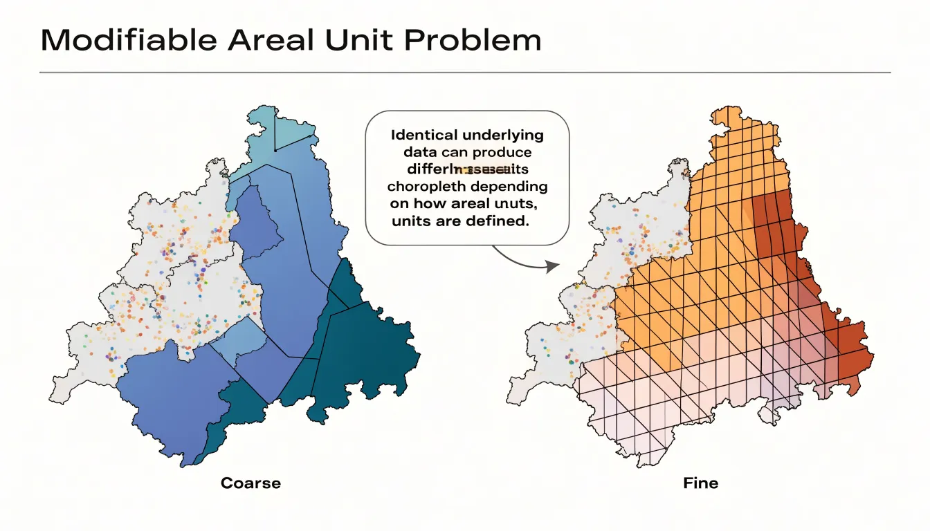
These boundaries are rarely neutral. Electoral districts, school zones, and municipal borders are often created for administrative or political purposes, not to reflect natural data distributions. When a choropleth map fills these shapes with color, it implicitly treats each region as homogeneous. In reality, populations and conditions vary within boundaries, and the placement of a line can either mask a pocket of high need or exaggerate a problem. A single tract might contain both affluent and disadvantaged neighborhoods, but the map assigns it one average value, smoothing over critical disparities.
Boundary changes over time compound the issue. Rezoning, annexation, or redistricting alters the shapes that choropleths depend on, making temporal comparisons unreliable. A map from one year may use different units than a map from the next, so apparent trends could simply reflect shifts in boundaries rather than real-world changes. This temporal instability can mislead decision-makers who rely on choropleths to track progress or allocate resources.
Normalizing Data
In choropleth mapping, raw counts—such as total population, number of cases, or total sales—are problematic because they are strongly influenced by the size and population of the underlying region. A large, densely populated region will almost always have high totals simply because it contains more people. When such totals are mapped directly, the largest regions dominate the visual story, suggesting they are the most affected areas even when their underlying rates are unremarkable.
To avoid this, choropleth maps require normalization: converting totals into rates, percentages, or per-capita metrics to adjust for the size of the population at risk. For example, mapping total disease cases makes large cities appear as hotspots, while mapping cases per 100,000 people reveals the true relative burden. Similarly, mapping total income highlights regions with many earners, whereas median household income or income per capita provides a more accurate picture of economic well-being.
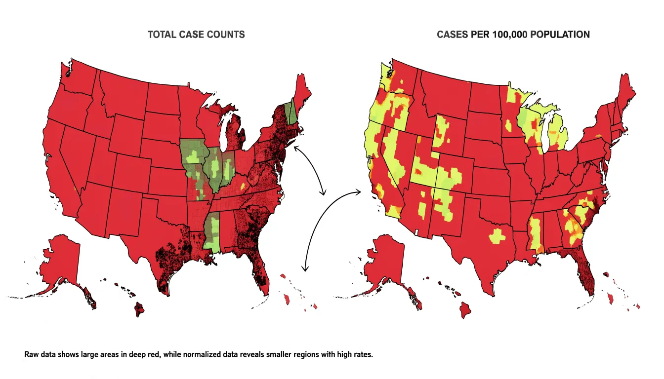
The choice of denominator should align with the question being asked. While population is common, other denominators such as land area, number of households, or number of facilities may be appropriate. Normalization ensures that the mapped value represents intensity or prevalence rather than sheer magnitude, preventing large regions from obscuring subtle patterns in smaller ones.
Ideal Heatmap Uses
Heatmaps excel in practical implementations where the goal is to track concentration and intensity across a continuous surface:
- Website user behavior: Click heatmaps aggregate thousands of user interactions to reveal where attention clusters on a page, which links draw the most taps, and which regions go untouched. Product teams use them to reposition calls to action, simplify navigation, and validate redesigns. Scroll-depth heatmaps extend the same logic vertically, showing how far down a page visitors travel before losing interest.
- Foot traffic tracking: Retailers, event organizers, and urban planners build heatmaps from sensors, Wi-Fi pings, or camera-derived counts to see how people move through a store, venue, or district. A shopping mall can identify which aisles attract lingering crowds and which remain cold spots to adjust layouts or signage. City agencies apply similar maps to pedestrian flows at transit hubs and public squares to plan crossings, place amenities, and manage peak-hour congestion.
- Meteorological observation: Weather agencies and forecasting platforms render temperature, precipitation, and storm intensity as color gradients that update as new readings arrive. Real-time heatmaps of rainfall or heat index let the public grasp where conditions are most severe and help forecasters communicate evolving patterns.
Ideal Choropleth Uses
Choropleth maps are best suited for data that is collected, reported, and analyzed within boundaries that carry legal, political, or statistical significance:
- Election results: Each voting district or county is colored according to the share of votes for a candidate or party. Because the boundaries correspond to where votes are counted and reported, the map directly reflects the underlying political geography, making it easy to spot regional strongholds, swing areas, and patterns of support.
- Economic indicators: Metrics like median household income are often mapped at the county, state, or census tract level. These units align with how economic data is collected and aggregated, allowing viewers to compare prosperity across recognizable regions.
- Demographic census statistics: Data on population density, age distribution, or racial composition fits naturally into census tracts and block groups. Because these units are designed to be stable over time and to contain relatively homogeneous populations, a choropleth map—such as the percentage of residents over 65—can reveal aging patterns and inform resource allocation in governance, public health, and urban planning.
Common Mapping Mistakes
Several recurring errors can distort spatial data across both map types:
- Plotting raw counts on choropleths: Mapping unadjusted totals—such as raw COVID-19 case counts by county—highlights populous areas regardless of actual infection rates. Always divide counts by a relevant denominator (population, area, or another base) to show true rates or ratios.
- Over-smoothing heatmaps: When the kernel density bandwidth is set too large, distinct clusters merge into a single blur and sharp local variations disappear, masking important hotspots or creating false continuities. Analysts should experiment with multiple bandwidths and validate results against the raw data. Additionally, when mapping discrete point data, using an appropriate color ramp and transparency helps avoid implying a continuous phenomenon where none exists.
- Perceptually uneven color steps: Palettes with uneven visual transitions, such as rainbow schemes, create false boundaries that lead viewers to perceive breaks not present in the data. Perceptually uniform palettes, like Viridis or ColorBrewer schemes, ensure that equal data intervals correspond to equal visual differences.
- Poor accessibility: Red-green combinations are problematic for colorblind viewers, and low-contrast palettes fail in grayscale or on poor displays. Using colorblind-safe palettes and testing legibility across devices ensures the map works for all audiences.
Choosing Your Map
Selecting between a heatmap and a choropleth map comes down to three factors:
- Dataset structure: Use a heatmap for raw point data (store addresses, event occurrences) where preserving the underlying distribution and revealing density clusters matters. Use a choropleth if your data comes pre-aggregated to regions (census tracts, counties, states) or if aggregating points to those regions is analytically meaningful.
- Spatial accuracy needs: Choose a heatmap when the goal is to highlight general trends and continuous surfaces rather than exact figures or borders, keeping in mind that it weights points equally but may imply data in empty areas. Choose a choropleth when precise regional comparisons and clear administrative boundaries are necessary, while accounting for the visual dominance of physically large regions.
- Target audience comprehension: Choropleth maps are familiar to most viewers and work well for public communication and policy discussions where regions are recognizable, reducing cognitive load when paired with clear legends and labels. Heatmaps are intuitive for showing intensity and suits exploratory analysis or technical audiences, though general viewers may need a brief explanation of how density is calculated and what the colors represent.
Overview
Modern GIS tools and libraries offer specialized environments for building both heatmaps and choropleth maps:
- Desktop platforms: QGIS and ArcGIS Pro provide full-featured environments for data preparation, styling, and export, suiting analysts who need precise control before publishing.
- Web-focused JavaScript libraries: Leaflet offers a lightweight entry point, Mapbox GL JS delivers polished vector rendering, D3.js supports custom data-driven visualizations, and deck.gl handles large datasets through GPU acceleration. OpenLayers and the Google Maps API are also popular for familiar basemaps and broad device support.
- Python libraries: Analysts working in Python often use Folium, GeoPandas, or Plotly.
Translating these tools into a usable map requires attention to interface design and performance. Legible legends should sit close to the map and explain color scales in plain language. Interactive features—such as hover tooltips, clickable regions, and zoom controls—let users explore detail at their own pace, while sensible defaults keep the initial view clear. For heatmaps, density should remain readable when zooming, which often requires dynamically adjusting radius and blur settings.
For large datasets, techniques like clustering, tiling, and progressive loading maintain responsiveness. Finally, responsive layout design, accessible color contrast, keyboard navigation, and text alternatives ensure the map remains usable across devices and audiences.
Frequently Asked Questions
What is the difference between a heatmap and a choropleth map?
A heatmap visualizes concentration and intensity across a continuous surface using plotted points and kernel density estimation, producing smooth gradients. A choropleth map divides an area into fixed, predefined units and shades each unit with a color representing an aggregated value, creating sharp boundaries between regions.
When should I use a heatmap instead of a choropleth map?
Use a heatmap for raw point data when preserving the underlying distribution and revealing density clusters matters, or when the goal is to highlight general trends and continuous surfaces rather than exact figures or borders. Use a choropleth if your data comes pre-aggregated to regions or if aggregating points to those regions is analytically meaningful.
What kind of data works best for a choropleth map?
A choropleth map is built for regional statistics assigned to an existing administrative or statistical area, such as a postal code, census tract, county, or district. These values often arrive as standardized metrics like rates, ratios, percentages, or indexes adjusted for area or population.
Why do choropleth maps need normalized data instead of raw counts?
Raw counts are strongly influenced by the size and population of the underlying region, so large, densely populated regions can dominate the visual story. Choropleth maps require normalization into rates, percentages, or per-capita metrics to show intensity or prevalence rather than sheer magnitude.
What is the Modifiable Areal Unit Problem in choropleth mapping?
The Modifiable Areal Unit Problem occurs because spatial analysis results can change significantly when the boundaries of the units used for aggregation are modified, even if the underlying data remain the same. These boundaries are rarely neutral and can mask or exaggerate conditions within a region.
What color schemes should I avoid for heatmaps and choropleths?
For heatmaps, rainbow palettes introduce perceptual distortions and are generally discouraged for precise data interpretation. For choropleths, using a continuous gradient can mislead viewers into thinking values change smoothly across boundaries, so a stepped color ramp with a limited number of classes is preferred.
Tony Astor
Tony writes about data visualization and the tools people use to build charts and dashboards. More about Data Illustrator