Flow Map: How to Visualize Movement Between Places
 By Tony Astor ·

Flow Map
A flow map is a spatial diagram that uses vector paths, node connections, and geographic anchors to represent the movement of people, goods, energy, or information between locations. Line width or color encodes volume, while arrowheads convey direction. Flow maps reveal corridors, hubs, bottlenecks, and origin-destination relationships across transit, logistics, migration, and tourism networks.
Table of Contents
Flow Maps
Flow mapping begins with the idea that movement has direction, volume, and geography. A flow map represents the transfer of something — people, goods, energy, information — between locations by combining a spatial base with symbolic marks that describe the movement itself. Its fundamental building blocks are vector paths, node connections, and geographical anchors.
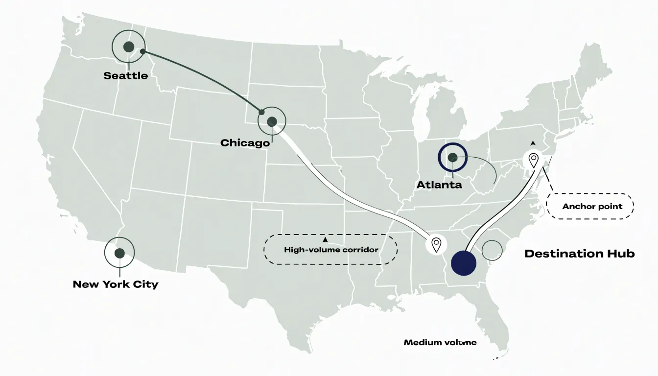
Vector paths are the visible strokes that carry the movement. Each path is drawn as a line or curve from an origin to a destination, and its geometry encodes direction. The path may be straight for simplicity or curved to suggest volume, avoid overlapping other paths, or follow a plausible route through space. Width or color along the path typically represents magnitude, such as the number of commuters, tons of freight, or units of energy transferred.
Node connections describe the relationships the paths express. Nodes are the points where flows begin, end, or pass through, and the connections between them form a network. A node can represent a city, a port, a facility, or an abstract region. The pattern of connected nodes reveals structure: which places act as hubs, which are peripheral, and how strongly locations are tied to one another. Read together, nodes and paths show both the individual movements and the overall network they compose.
Geographical anchors tie the diagram back to real space. Anchors are the positions of nodes on the underlying map, whether that map is a precise projection, a schematic layout, or an abstract canvas. They give flows their spatial context, so a wide path between two locations can be interpreted as traffic between specific places rather than as a purely abstract quantity. Together, vector paths, node connections, and geographical anchors form the basic grammar of spatial flow mapping.
Origin-Destination Pairings
Origin-destination (OD) pairings define the relationships between where movement begins and where it ends. Structuring OD data effectively starts with a clear matrix layout: rows represent origins, columns represent destinations, and each cell holds a value such as trip count, volume, or intensity. This matrix format ensures that every possible pairing has a designated place, making it easy to compute totals, identify dominant flows, and spot imbalances. For large datasets, aggregating locations into zones or regions keeps the matrix manageable and interpretable.
When drawing connecting vectors, use consistent line styles and colors to represent magnitude or direction. Ensure that lines are drawn with slight curves or offsets to avoid overlapping and to distinguish between bidirectional flows.
Labeling is also critical: place origin and destination labels near their respective points, using leader lines or callouts if necessary. For dense maps, interactive elements or filtering options can help users explore specific OD pairs without overwhelming the visual. Always include a legend that explains line thickness, color scales, and any symbology used.
Finally, validate your OD matrix for completeness and accuracy. Check for missing data, ensure that origins and destinations are consistently geocoded, and verify that flow totals align with known benchmarks.
Line Weight
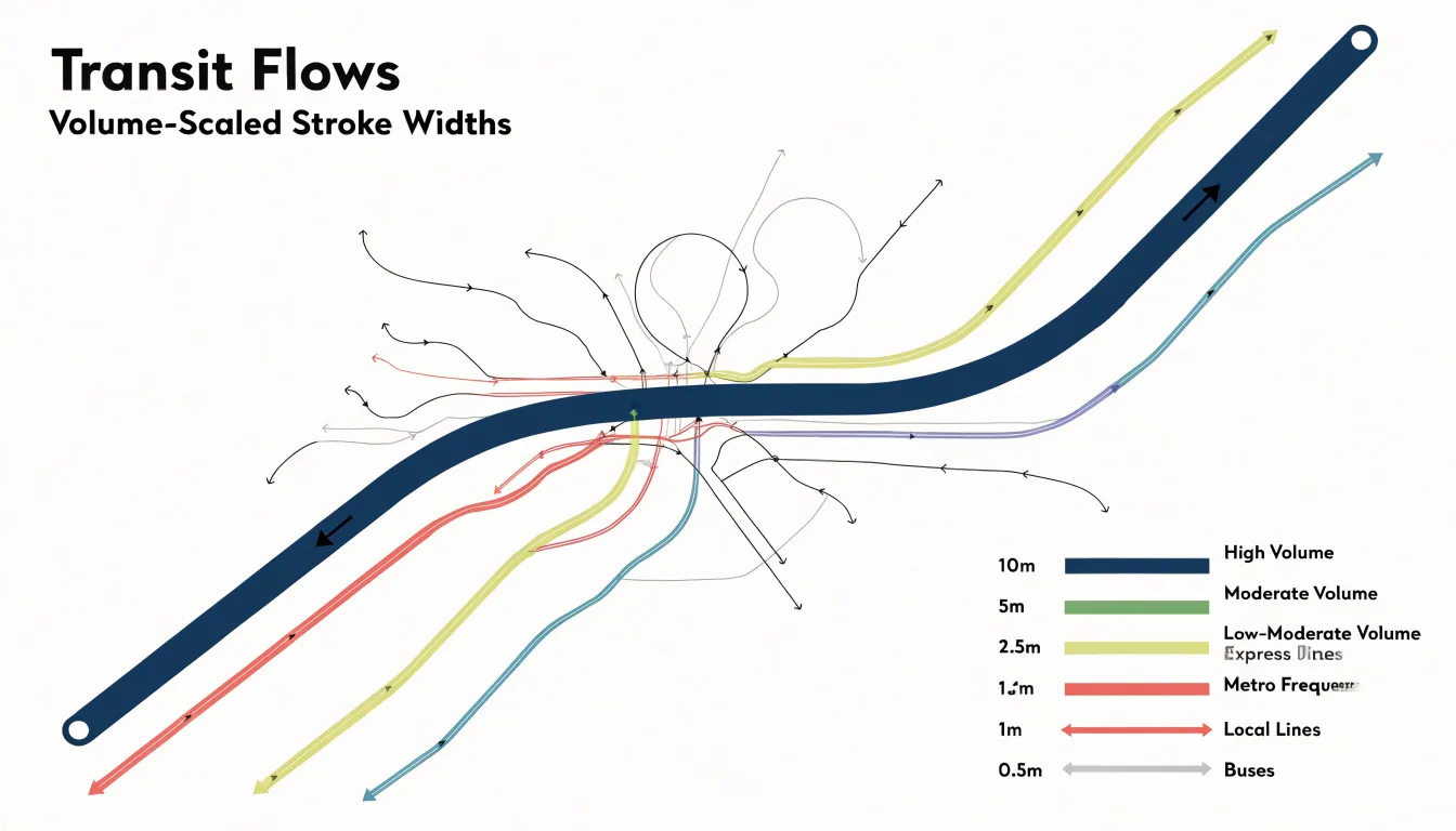
By scaling stroke width proportionally to quantitative volume data, a flow map encodes traffic density directly into the geometry of each route. A thick stroke draws the eye first, signaling a high-volume corridor, while a thin stroke recedes, indicating lighter use. This proportional scaling creates a visual hierarchy that viewers can parse quickly to identify major arteries and secondary routes.
The relationship between stroke width and volume must be carefully calibrated. A linear scale often works well for moderate ranges, but when volumes vary widely, a square-root or logarithmic scaling can prevent extreme values from dominating the map while still preserving relative differences.
In transit maps, this technique is particularly effective for showing capacity: a thick line might represent a subway line with frequent, high-capacity service, while a thin line could indicate a less frequent bus route. Moreover, line weight interacts with other map elements, such as color and labels, to reinforce the message and convey density across a region.
Directional Arrows
Directional arrows answer a simple question—which way?—without stealing attention from the data itself. The most common technique is the arrowhead, placed at the destination end of a line. The key is restraint: arrowheads should be proportional to line thickness, large enough to read at a glance but small enough to avoid clutter. For curved paths, orient the arrowhead tangent to the line’s final segment so it follows the natural curve. When many lines converge, consider placing arrowheads at consistent intervals along the path rather than only at the terminus, giving viewers multiple cues without repetition.
Animated particles offer a dynamic alternative. By moving small dots or dashes along a path, you can convey direction and relative speed simultaneously. Keep the animation subtle: slow, steady motion reads as informative, while rapid or flashing particles become distracting. Limit animation to a few key routes or use it sparingly in interactive versions where users can pause or scrub through the flow.
Tapered lines provide a static solution. By gradually narrowing a line from source to destination, the taper itself implies direction—wider at the origin, narrower at the end—while also encoding magnitude through width. The taper should be smooth and consistent, as abrupt changes in width can confuse the eye.
Across all techniques, use a single directional cue per line, maintain consistent sizing, and let the map’s overall hierarchy guide where arrows appear.
Color Coding
Color coding allows viewers to distinguish categories of movement at a glance before engaging with labels or legends. When a transport network carries multiple modes—rail, road, air, and water—assigning each a distinct color palette creates instant visual separation, so a viewer tracking a rail corridor can follow it across the map without losing it among overlapping highway routes. The same principle applies to freight: cargo types such as bulk goods, perishables, hazardous materials, or containerized shipments can each receive their own hue, showing where particular commodity flows concentrate and how they intersect with other supply chains.
Temporal shifts add a further dimension. By varying color intensity or shifting palettes across time periods, a flow map can show how traffic patterns change from morning to evening, weekday to weekend, or season to season, with lighter tones indicating off-peak movement and deeper saturation marking periods of heaviest volume.
The effectiveness of these choices depends on careful palette design. Colors must remain distinguishable from one another—including for viewers with color vision deficiencies—and must hold up against the map’s background tones. Palettes with strong hue separation and consistent value contrast tend to work best, particularly when many categories appear simultaneously. Consistency across a series of maps matters as well: a color assigned to one mode or commodity should retain that association throughout a document or dashboard so readers can compare panels without relearning the key each time.
Commuter Routes
Commuter routes carry large volumes of passengers between residential suburbs and urban employment centers on a predictable daily rhythm. Mapping these patterns begins with assembling reliable origin-destination data, typically drawn from fare card records, automatic passenger counters, and household travel surveys. Each record captures where a journey starts, where it ends, and when it occurs, allowing analysts to reconstruct the shape of the morning and evening peaks with precision. Cleaning and geocoding these records is an essential first step, since inconsistencies in station names or stop identifiers can distort the resulting picture.
Once the data is prepared, flow maps with lines scaled to passenger volume reveal which suburban-to-urban corridors carry the heaviest loads and where capacity constraints are likely to emerge. Desire lines drawn between home and workplace zones offer a complementary view, showing the straight-line demand that existing rail or bus networks may only partially serve. Layering peak-hour volumes over the base network highlights the concentration of travel into narrow time windows, making the case for additional service during rush periods.
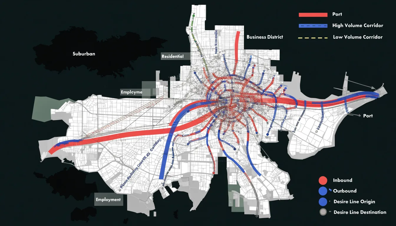
To capture the temporal dimension, animating flows across the morning and evening peaks can show how corridors reverse direction between the two periods, while small multiples of hourly snapshots expose the gradual buildup and dispersal of demand. Color ramps that differentiate inbound from outbound movement help readers distinguish the two directions without ambiguity. Combining these approaches helps planners, transit agencies, and policymakers anticipate how shifts in remote work or housing development might reshape the daily commute over time.
Supply Chain Logistics
Supply chain logistics depends on tracing multi-modal freight routes across road, rail, air, and sea from factories to stores. A typical journey begins at a manufacturing plant, where finished goods are loaded onto trucks or rail cars for the first leg of the trip. From there, cargo may move to a port terminal, cross an ocean lane aboard a container ship, and transfer again to regional distribution centers before reaching individual retail locations. Mapping each of these handoffs shows where goods consolidate, where they wait, and where they disperse into local delivery fleets.
Distribution bottlenecks appear naturally when these routes are drawn together. A port that handles a disproportionate share of container traffic, a single highway corridor serving several warehouses, or a rail junction where multiple lines converge can all become points of congestion that ripple outward through the entire chain. Flow maps highlight these pressure points by showing the volume of goods passing through each node relative to its capacity, allowing analysts to spot chokepoints before they cause delays.
Global shipping lanes form the long-distance backbone of this network. Major maritime corridors connect manufacturing hubs in Asia, Europe, and the Americas, and the maps trace how container traffic funnels through straits, canals, and transshipment ports. Visualizing these lanes alongside inland freight routes reveals the full path a product travels. Planners use this perspective to evaluate alternate routes, balance loads across transport modes, and anticipate how disruptions at a single point—such as a blocked canal or a strained port—will propagate through the wider system.
Migration Patterns
At the macro level, migration visualizations capture the slow reshaping of continents: rural populations draining toward coastal cities, labor moving from one economic zone to another, and families following opportunity across borders. The width of a line measures how many people made the same journey, while its length speaks to the distance they crossed.
Historical migration vectors add a temporal dimension to this picture. By layering flows from different eras, a map can show how routes persisted, shifted, or reversed over decades. Trade corridors that once carried merchants may later carry refugees, and settlement patterns established centuries ago can still shape where populations cluster today. Visualizing these layers side by side, or in sequence, reveals continuities that are otherwise invisible in a single snapshot.
Displaced population shifts present a more urgent application of the same technique. When conflict or environmental change forces people from their homes, flow maps trace the movement of large groups across regional boundaries, often under conditions where data is scarce and rapidly changing. Here the map serves not only as analysis but as documentation, recording the scale and direction of displacement for policymakers, aid organizations, and the historical record.
Tourist Movement
Visitors to popular cities leave behind detailed traces of where they go, how long they linger, and which routes they choose between landmarks. Aggregated location data—drawn from mobile networks, app usage, and public transport taps—allows researchers to reconstruct these paths at scale while preserving individual anonymity. The resulting picture shows how visitors distribute themselves across a city over the course of a day, revealing corridors that connect major attractions and quieter streets that see only occasional footfall.
Landmark density hotspots emerge clearly from this tracking. Certain intersections, squares, and museum districts accumulate disproportionate numbers of visits, forming nodes where pedestrian traffic thickens and where local services, transport links, and public space come under pressure. Mapping these hotspots helps city planners see where crowding may degrade the visitor experience.
Seasonal pedestrian journeys add a temporal dimension to the analysis. Grouping data by time of year reveals shifts such as summer crowds concentrating along waterfronts or winter visitors clustering around indoor cultural sites. Similarly, comparing spring and autumn movement patterns, or weekday and weekend flows, shows how the rhythm of tourism reshapes a city’s streets. Some routes appear only during peak holiday periods, while others remain stable year-round and may reflect the movement of residents as much as visitors. Tracing these journeys supports decisions about signage and the placement of temporary facilities, while highlighting quieter zones where planners might encourage a more even distribution of visitor activity.
Radial Flow Layouts
Radial flow layouts organize movement around a single dominant hub, with flow vectors radiating outward toward the periphery. Every route, line, or vector originates from or terminates at one major node, and all secondary destinations are reached by passing through that center. A major international airport illustrates the principle well: passengers traveling between regional cities typically connect through the central hub rather than flying directly to one another, and the route structure fans out like spokes from the axle of a wheel. A central freight terminal operates on the same logic, gathering shipments from many surrounding origins into one consolidation point before dispatching them outward to their final destinations.
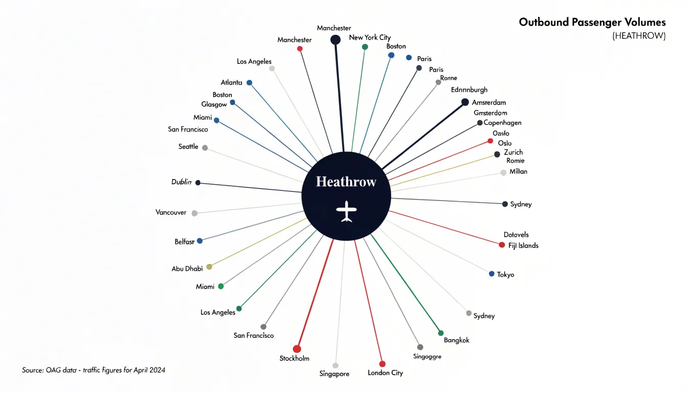
This arrangement concentrates activity and infrastructure at the hub, making the center the busiest and most heavily invested part of the system. The peripheral points remain relatively simple, each connected by a single path to the center, while the hub must handle the full volume of traffic passing through the network. Visually, the eye is drawn immediately to the central node, and the density of lines around the hub communicates its importance without additional labeling.
Radial layouts suit systems where one location genuinely dominates demand or supply, such as a capital city with a centralized rail network or a port serving a wide hinterland. The pattern also reveals vulnerability, since disruption at the central hub can affect every route in the system simultaneously. When drawing flow maps, the radial approach offers a compact, legible way to represent many-to-one and one-to-many relationships.
Network Flow Diagrams
Network flow diagrams represent transit systems where dozens of routes share the same physical space. In a dense urban grid, buses, rail lines, and pedestrian corridors frequently converge on the same intersections, then diverge again in different directions. A network flow diagram captures these interactions by treating the shared geographic grid as a stable reference frame and layering the intersecting travel paths on top of it. Each node marks a point of contact: a station, a transfer point, or a junction where paths split or merge. Edges connect these nodes and carry directional weight, showing how traffic moves through the network rather than merely where the lines run.
Complex web-like networks demand careful handling of overlapping segments. When several routes traverse the same corridor, the diagram can bundle them into a single band whose width or shading reflects the combined volume, then fan them out as they approach a divergence point. Split nodes show where a corridor divides into separate branches, while merge nodes show where branches rejoin. This structure lets a reader trace a single journey across the map while also seeing how that journey relates to the wider system.
While the shared geographic grid keeps the diagram grounded in recognizable streets, districts, and landmarks, the diagram prioritizes topology over exact scale. This clarifies connections that would otherwise be obscured by geographic clutter, scaling from a handful of intersecting lines to a full metropolitan web.
Avoiding Visual Clutter
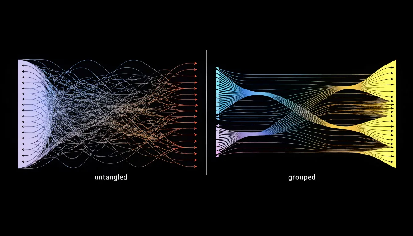
Dense flow maps frequently accumulate overlapping lines wherever many routes converge on shared destinations or pass through narrow corridors, obscuring the underlying structure of the data. Three techniques work together to keep these dense networks legible:
- Edge bundling groups related flow paths into shared trajectories. Instead of dozens of separate strands crossing the same region, the viewer sees a small number of thicker bundles that separate again as they approach their endpoints, preserving overall direction and volume while removing visual noise.
- Line transparency lets individual paths fade where they crowd together, so the eye can register density without being overwhelmed by solid strokes layered on top of one another. Lighter, semi-transparent strokes allow underlying patterns to remain visible even in the busiest areas of the map.
- Path curvature makes individual routes easier to trace than straight segments that cut across one another. Gently arcing lines give each flow a distinct visual signature and can be routed around congested zones rather than through them.
Common Mapping Mistakes
Many of the most common mistakes in flow mapping stem from treating the map as a static picture rather than a quantitative instrument:
- Unscaled line weights: When the thickness of each flow line is chosen by eye rather than tied to a consistent formula, viewers cannot compare routes reliably; a modest corridor may appear dominant simply because someone liked the look of a thicker stroke. Scale line width proportionally to the underlying value, keep the scaling consistent across the whole map, and provide a legend showing how widths correspond to actual magnitudes.
- Busy background basemaps: Detailed satellite imagery or richly labeled street networks compete with the flow lines for attention, burying the data under visual noise. Use a muted, low-contrast basemap—stripping unnecessary labels, reducing saturation, and lightening the underlying terrain—so the flows read as the primary subject while retaining geographic context.
- Poor color choices: Rainbow palettes rarely convey ordered meaning, and adjacent colors of similar lightness become indistinguishable at small sizes or for color-vision-deficient readers. Use sequential palettes for flows ordered by magnitude, and categorical hues for genuinely distinct groups. Equally important, line color should never fight the basemap; a saturated flow line over a saturated background produces vibration and fatigue.
- Confusing layouts: Lines that overlap ambiguously, cross without clear separation, or cluster near nodes make individual routes hard to follow. Careful routing, subtle casing around lines, and deliberate ordering of overlapping flows keep the network legible.
Storytelling With Flow Maps
Transforming raw trajectory data into a coherent narrative begins with aggregating individual paths of coordinates to reveal collective flows. While dominant corridors highlight major trends, anomalies—like divergent paths or unexpected detours—stand out as visual outliers that prompt further investigation.
By layering contextual data, such as time of day or environmental conditions, the map evolves into a dynamic narrative that explains why flows occur. Spatial relationships, including convergence points and bottlenecks, become focal points showing how locations interact. Supported by a clear visual hierarchy, intuitive legends, and interactive elements for exploring details, these maps translate abstract trajectory points into a clear view of the hidden rhythms of movement.
Practical Applications
Flow maps give urban planners and transit authorities a practical instrument for optimizing public transportation routes. By tracing the paths of commuters, buses, trains, cyclists, and pedestrians, planners see where demand concentrates and where it thins out. When a corridor shows a heavy, steady stream of riders, agencies can justify adding service, adjusting schedules, or introducing express lines. When a route shows sparse, erratic movement, planners gain evidence for rerouting or consolidating services to reduce waste and improve coverage elsewhere.
The same visual logic supports infrastructure design. Flow maps reveal pinch points where many paths converge and slow down, such as crowded transfer stations, narrow bridges, or intersections with heavy turning traffic. Seeing these bottlenecks mapped out helps engineers prioritize where to widen a road, add a dedicated bus lane, build a pedestrian crossing, or redesign a junction. Because the maps show direction as well as volume, they also expose directional imbalances—such as morning flows surging inbound and evening flows reversing—which informs decisions about one-way systems, reversible lanes, and peak-hour management.
Transit authorities also use flow maps to communicate with the public and decision-makers, turning abstract ridership statistics into an intuitive picture that residents, councillors, and funding bodies can grasp quickly to build support for projects. Finally, planners layer flow data with land-use information to anticipate how new housing, workplaces, or commercial districts will generate traffic, allowing infrastructure to be designed ahead of demand rather than scrambled together afterward.
Frequently Asked Questions
What are the main components of a flow map?
Flow maps are built from vector paths, node connections, and geographical anchors. Vector paths carry movement, node connections describe relationships, and geographical anchors tie the diagram to real space.
How do you set up an origin-destination matrix?
Use rows for origins, columns for destinations, and each cell for a value such as trip count, volume, or intensity. For large datasets, aggregate locations into zones or regions to keep the matrix manageable and interpretable.
How should line thickness be used in a flow map?
Scale stroke width proportionally to quantitative volume so thick strokes signal high-volume corridors and thin strokes indicate lighter use. For moderate ranges a linear scale often works, while square-root or logarithmic scaling can prevent extreme values from dominating when volumes vary widely.
What is the best way to show direction on a flow map?
Place an arrowhead at the destination end, keep it proportional to line thickness, and orient it tangent to curved paths. You can also use subtle animated particles or tapered lines, but use a single directional cue per line.
How are flow maps used in supply chain logistics?
Flow maps trace multi-modal freight routes across road, rail, air, and sea from factories to stores, showing where goods consolidate, wait, and disperse. They also highlight bottlenecks by showing the volume of goods passing through each node relative to its capacity.
How can I reduce visual clutter in a dense flow map?
Use edge bundling, line transparency, and path curvature to keep dense networks legible. Edge bundling groups related paths into shared trajectories, transparency lets crowded paths fade, and curvature makes individual routes easier to trace.
Tony Astor
Tony writes about data visualization and the tools people use to build charts and dashboards. More about Data Illustrator