Famous Data Visualizations and What They Teach Us
 By Tony Astor ·

Famous Data Visualizations and What They Teach Us
John Snow’s 1854 Broad Street pump map plotted cholera deaths by street address, revealing a cluster around one contaminated water pump and founding modern epidemiology. Florence Nightingale’s polar area diagrams, Minard’s flow map, Beck’s topological tube map, Playfair’s bar and line charts, and the Isotype system show that chart type is a rhetorical decision: matching visual form to the reader’s task can turn data into evidence that changes policy and public understanding.
Table of Contents
Chart Type
In 1854, a cholera outbreak swept through London’s Soho district, killing hundreds of residents in days. At the time, the prevailing theory held that disease spread through miasma—foul air arising from decaying matter. Dr. John Snow, skeptical of this explanation, suspected the illness was transmitted through contaminated water. To test his hypothesis, he plotted each death as a bar mark on a street map of the neighborhood. The resulting visualization, now known as the Broad Street pump map, revealed a striking pattern: fatalities clustered densely around a single public water pump on Broad Street, radiating outward as distance from the pump increased. Snow’s map transformed a chaotic public health crisis into legible spatial evidence.
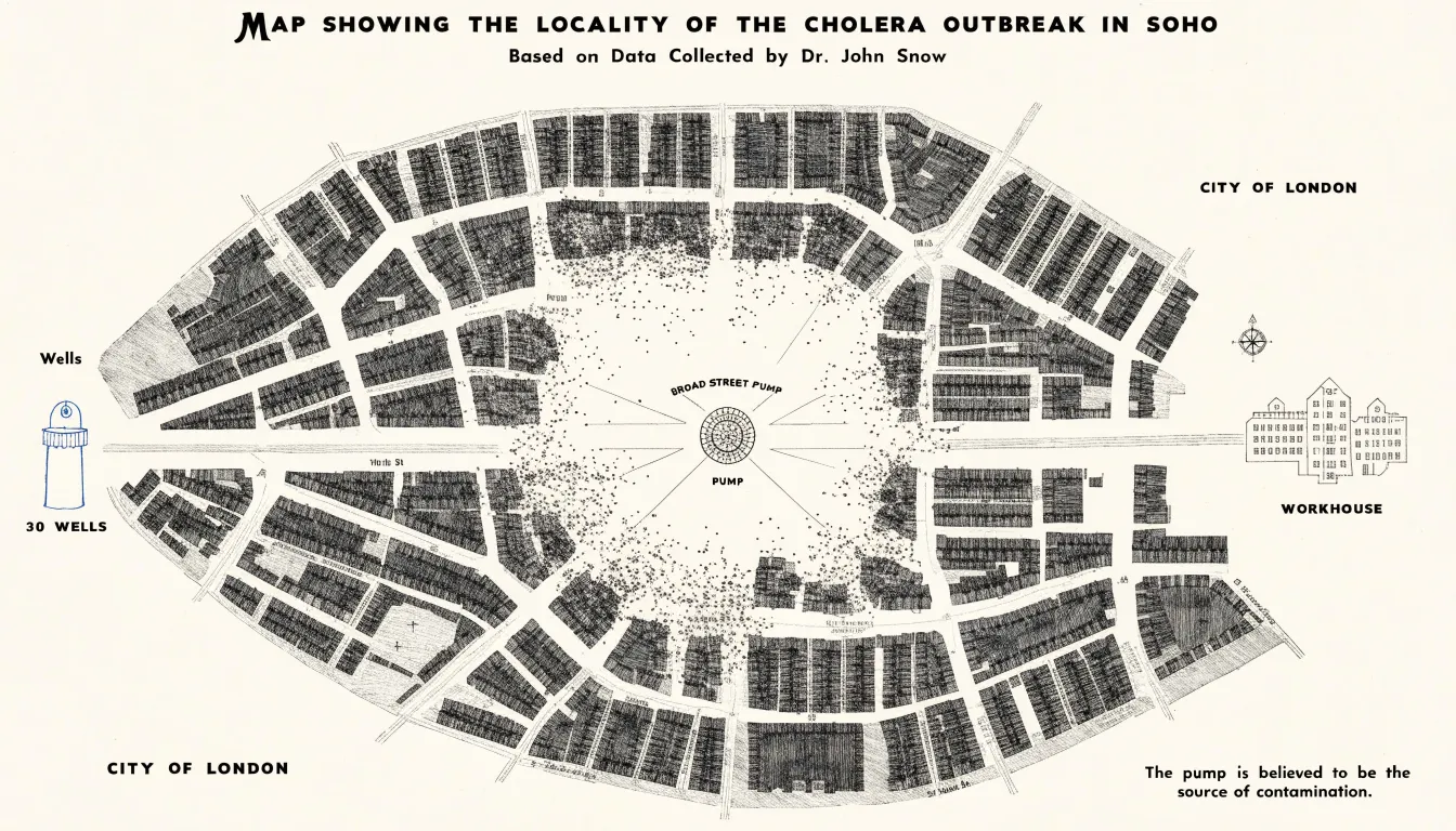
The design choices behind the map matter as much as its conclusion. By anchoring each death to a precise street address, Snow let the geographic distribution speak for itself, allowing viewers to trace the concentration of marks toward the pump without statistical training. He also annotated anomalies that a casual glance might miss, such as a workhouse and a brewery whose residents escaped the outbreak because they drew water from their own wells. These details reinforced the pattern and preempted counterarguments.
Snow’s map is widely regarded as a foundational moment in epidemiology, demonstrating that plotting health data in geographic space can reveal causal relationships invisible in tables of numbers. Modern disease surveillance systems, from outbreak dashboards to contact-tracing tools, descend directly from this approach, showing how a carefully constructed graphic can challenge accepted wisdom and change the course of public health.
Chart Type
Florence Nightingale’s polar area diagram, often called a rose diagram, stands as one of the most consequential chart choices in the history of data communication. During the Crimean War, Nightingale collected meticulous records on the causes of soldier mortality. Her analysis revealed a stark pattern: far more British soldiers were dying from preventable diseases contracted in unsanitary hospital conditions than from battlefield wounds.
Knowing that an ordinary table would bury this insight in rows of numbers, Nightingale worked with statistician William Farr to render the data as a series of equal-angle wedges. The area of each wedge represented monthly death counts, colored to distinguish deaths from disease, wounds, and other causes. Published in her 1858 report on the health of the army, the resulting diagrams made the overwhelming share of disease-related deaths visible at a glance. Each wedge’s size communicated proportion immediately, and the colored segments allowed viewers to compare causes across months without decoding a legend-heavy table.
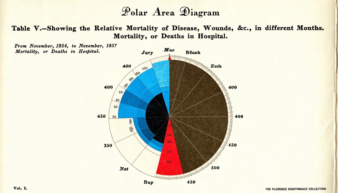
This visual framing gave Nightingale a persuasive instrument to place before ministers, parliamentarians, and Queen Victoria. The pressure generated by the diagrams contributed to the establishment of the Royal Commission on the Health of the Army and sweeping sanitary reforms in military and civilian hospitals. For leaders working with data today, the lesson is that chart type is itself a rhetorical decision. Choosing a form that maps magnitude to visible area and directs attention to the comparison that matters can turn a spreadsheet into an argument that changes policy.
Chart Type
Charles Joseph Minard’s 1869 map of Napoleon’s Russian campaign demonstrates the power of a flow map to integrate multiple variables into a single coherent drawing. The map depicts the dramatic reduction of Napoleon’s army as it advanced toward Moscow and retreated, using a continuous band whose width represents troop strength. This band narrows steadily from 422,000 men at the start to just 10,000 at the end, making the catastrophic loss immediately visible.
Beyond troop size, Minard incorporates five other variables:
- Geography and location: The army’s route is traced across a map of Russia, with rivers and cities providing spatial context, including the splitting and rejoining of troops and the devastating final crossing of the Berezina River.
- Direction of movement: The color of the band (tan for advance, black for retreat) and the flow of the shape itself show the path forward and back.
- Temperature and time: A line graph below the main map tracks the bitter cold during the retreat, showing values like -30 degrees Réaumur tied to specific dates and locations.
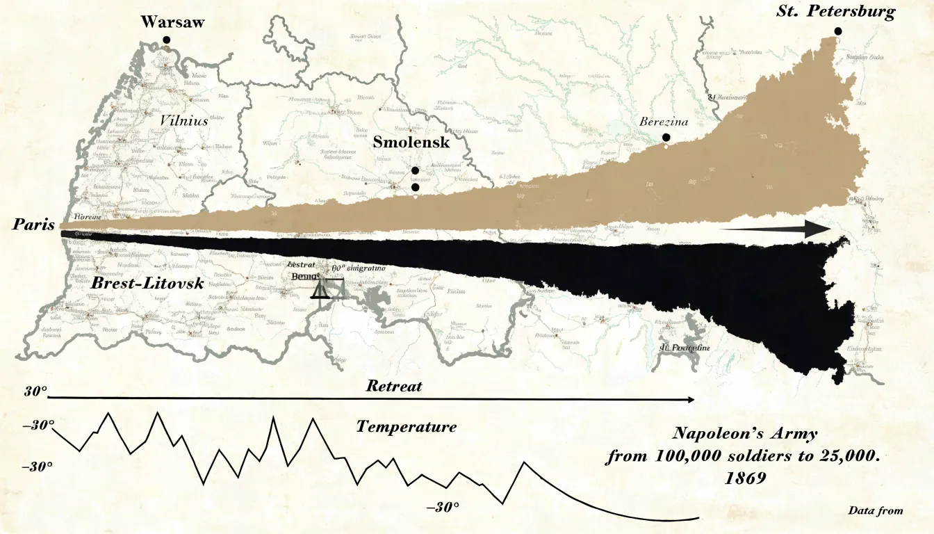
By layering geography, troop strength, direction, temperature, time, and location, Minard created a narrative that is both informative and emotionally powerful. The flow map remains a premier model for showing movement and multivariate change over space and time.
Chart Type
W.E.B. Du Bois approached the 1900 Paris Exposition with a clear purpose: to show the world, through data, the true condition of Black Americans forty years after emancipation. Working with a team of students at Atlanta University, he assembled more than sixty hand-drawn charts and graphs, now celebrated as the Exhibit of American Negroes. Among the most striking were bold graphics rendered in vivid reds, greens, yellows, and blacks, arranged in clean geometric forms that filled entire poster boards. Spirals, stacked bars, and segmented rectangles replaced the dense tables typical of nineteenth-century statistics.
The subject matter was deliberately dual. The charts documented real progress—including rising literacy rates, property ownership, and enrollment in higher education—while also mapping the systemic barriers that constrained Black life. One famous spiral chart traced the growth of the Black population over decades, its widening arc conveying scale and momentum. Others compared landownership, occupational categories, and the distribution of professions across states, revealing how exclusion from education, credit, and civil institutions produced measurable inequality. Du Bois used color not as decoration but as an analytical tool, grouping categories so that patterns of disadvantage and advancement became immediately legible to an international audience.
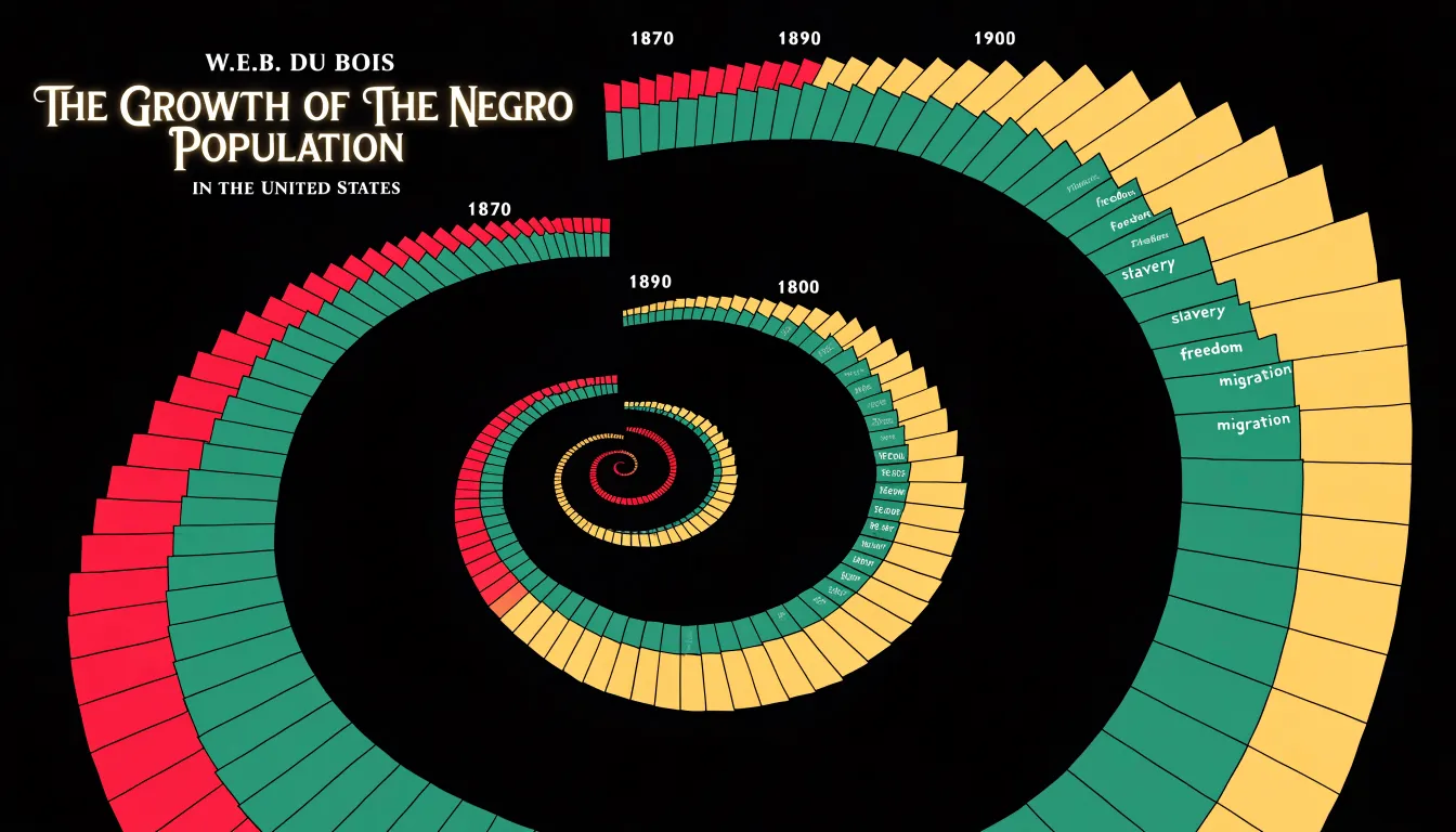
These visualizations demonstrate how design choices carry argumentative weight. Strong color and geometry made the data accessible to lay viewers, and the sheer ambition of the collection asserted Black intellectual capacity in a period when that capacity was widely denied. Du Bois’s exhibit shows that clarity, beauty, and moral purpose can operate together, serving both explanation and advocacy.
Chart Type
Harry Beck’s 1933 map of the London Underground teaches a core lesson about the relationship between a chart’s purpose and its fidelity to the physical world. Before Beck, transit maps attempted to show routes as they actually ran across the city, winding through streets and following the real contours of the rail lines. These maps were geographically faithful, yet passengers struggled to read them. Beck, an engineering draftsman who worked on the Underground in his spare time, recognized that travelers rarely need to know the true distance or direction between stations. They only need to know which line to take, where to change, and how many stops remain.
Working from that insight, Beck straightened the tangle of routes into horizontal, vertical, and forty-five-degree lines. He spaced stations evenly along each line, exaggerating the central area where stops cluster closely in reality and compressing the outer reaches where they are far apart. The River Thames became a stylized reference mark rather than a surveyed watercourse. Geography gave way to topology: what mattered was the order of stations and the points where lines intersect.
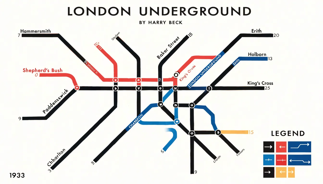
Passengers could now trace a journey, count stops, and spot the correct interchange without decoding a cluttered picture of the city. The approach proved so effective that it became the template for transit maps worldwide, from Tokyo to New York. The broader lesson for chart designers is that physical accuracy is a means rather than an end. Deliberate simplification, guided by a clear understanding of the reader’s task, often communicates far more effectively than a literal rendering of reality.
Chart Type
Animated bubble charts combine three or more dimensions of data within a single moving display. Each bubble carries a horizontal position, a vertical position, a size encoding a third variable, and often a color that distinguishes categories or regions. When set in motion across a time axis, the chart can display decades of change in seconds. Hans Rosling’s Gapminder presentations demonstrated this potential by plotting income per person against life expectancy for every country in the world, with bubble size reflecting population. As the animation advanced year by year, viewers watched nations drift across the plane, clusters break apart, and trajectories diverge.
The power of this format lies in its capacity to overturn entrenched assumptions through direct observation. Rosling designed his animations to challenge widespread beliefs about the developing world, showing that many countries conventionally labeled as poor had achieved substantial gains in health and prosperity. The motion itself carried the argument, since a static snapshot of any single year could not convey the pace or direction of change. Viewers saw life expectancy climbing and income rising in tandem across large parts of Asia and Latin America, contradicting narratives of stagnation. When tied to meaningful variables, motion can make complex global trends legible to broad audiences and reframe how people understand the world.
Chart Type
Ed Hawkins introduced the warming stripes in 2018 to communicate decades of climate data through color alone. Each stripe represents a single year, arranged chronologically from left to right. Its hue is drawn from a sequential palette that shifts from cool blues for cooler-than-average years through neutral tones toward deep reds for the warmest years on record. The chart carries no axes, gridlines, labels, or numerical values. This deliberate minimalism removes the barriers that often separate general audiences from scientific data, allowing a viewer to perceive the long-term warming trend within seconds.
The sequential color scale does the heavy lifting in this design. Because the palette progresses along a single perceptual dimension from cool to warm, viewers read the stripes as a continuous gradient rather than as discrete categories. The eye naturally groups adjacent stripes and registers the shift from predominantly blue years on the left to predominantly red years on the right. This encoding exploits a deep cultural association between blue and cold, and between red and heat, so the meaning lands instinctively. Stripping away numbers also sidesteps the interpretive friction that statistics can create, letting the visual pattern speak directly to intuitive understanding.
Adapted for countries, cities, and regions worldwide, the warming stripes have appeared on clothing, public buildings, and social media in enormous numbers. Their success demonstrates that when the central message of a dataset is a long-term directional trend, a simple sequential visual can travel far beyond specialist audiences and communicate more powerfully than a detailed line chart.
Chart Type
William Playfair, a Scottish engineer and political economist, is widely credited with inventing several fundamental chart types in the late 18th century. His 1786 work, The Commercial and Political Atlas, introduced the bar chart and the line graph as tools for understanding economic data, which had previously been locked in dense tables requiring mental calculation to interpret.
Playfair used bar charts to display the balance of trade between England and other nations, with bars of different lengths representing imports and exports so readers could quickly compare trade flows and identify surpluses or deficits. His line graphs tracked economic trends over time, such as the price of wheat or the national debt. By connecting data points with lines, Playfair showed how values changed across years, making fluctuations and long-term patterns immediately visible.
These innovations shifted the focus of data presentation from precise numerical lookup to broader trends and comparisons, enabling policymakers and merchants to grasp economic conditions rapidly. Playfair’s work laid the foundation for modern data visualization, and line and bar graphs remain among the most common chart types today.
Chart Type
Otto Neurath and Marie Reidemeister developed the Isotype system during the 1920s and 1930s to solve a specific communication problem: how to present quantitative information to audiences with different languages and varying levels of literacy. Working in Vienna and later in exile in the Netherlands and Britain, the pair built a visual language around repeated symbols, where each icon represented a fixed quantity of a given item. A row of simplified human figures might stand for a population; a stack of stylized barrels might represent oil production. The symbols were standardized so viewers could count them, compare rows, and grasp relative magnitudes without reading a single word of explanatory text.
The system grew out of Neurath’s philosophical interest in the unity of science and the idea that visual communication could serve as a universal medium. Reidemeister, who later married Neurath and worked alongside him for decades, handled much of the practical design work, refining the iconography and the rules governing how symbols were scaled, repeated, and arranged. Their collaboration produced charts for museums, exhibitions, and publications, including the Social and Economic Museum of Vienna and later the Isotype Institute in Oxford.
Isotype charts prioritize the reader’s context over the designer’s preferences, choosing pictorial clarity when text would exclude part of the audience. Their insistence on consistent symbol sizes and repeated units also anticipated modern concerns with proportional representation. When a single symbol is scaled up in size to show growth, viewers often misread the change in area; the Isotype rules guarded against this distortion by treating each icon as a fixed unit to be repeated rather than a stretchable shape.
Chart Type
Small multiples offer a disciplined way to compare complex trends by repeating a single graphic structure across a grid of panels. Each panel shares the same axes, scale, and visual encoding, so the only thing that changes from one frame to the next is the variable under examination. Once readers understand one panel, they understand the grammar of them all, and their attention shifts from decoding the chart to comparing the patterns within it. Edward Tufte popularized this framework as a way to display multivariate data with economy, allowing viewers to see variation across categories, time periods, or conditions without overlaying dozens of lines on a single canvas.
The value of small multiples lies in how they manage cognitive load. A single chart crowded with overlapping series forces readers to track colors, labels, and legends while disentangling crossed lines. Repeating simple graphics instead lets the eye move across panels and register differences in slope, level, or volatility almost immediately. Because the design stays constant, any deviation stands out as meaningful, and readers can hold several patterns in mind at once without losing their place.
This approach suits data with a natural categorical structure, such as regions, products, or demographic groups tracked over time. The grid itself becomes part of the argument, revealing clusters of similar behavior and outliers that a combined chart would obscure.
Chart Type
The hockey stick graph, first published by Michael E. Mann and colleagues in the late 1990s, remains one of the most recognizable images in climate science. The chart plots reconstructed Northern Hemisphere temperatures across roughly six centuries and overlays instrumental records for the most recent decades. A single continuous line traces this history, running flat and steady through the centuries before bending sharply upward in the twentieth century.
By reducing a complex model—built from tree rings, ice cores, corals, and instrumental records—into one visual element, the chart makes the trajectory immediately clear to non-specialists. The long flat handle of the stick establishes a historical baseline against which the recent spike can be judged, so the final upward turn reads unmistakably as a departure from a known norm.
Its influence also highlights the responsibilities that come with such simplification. A single line smooths over uncertainty ranges, regional variation, and the many data sources behind the reconstruction—details that appear in the underlying papers but often fade in the popular reproduction of the image. Later studies refined the curve and critics debated its methods, yet the visual remained a touchstone in public discussion of climate change. Choosing one line to represent a complicated model can make findings legible to millions, provided the presentation accounts for what has been condensed into that line.
Chart Type
Spatial heat maps have transformed decision-making in professional sports by aggregating thousands of individual data points—such as the location of every shot attempt or the coordinates of each player throughout a game—into a color-coded grid overlaid on a playing surface. Warmer colors signal dense clusters of activity, while cooler tones show sparse areas. This two-dimensional plane divided into zones lets coaches and analysts absorb the overall shape of a team’s behavior before drilling into specific regions.
In basketball, shot charts built on this model reveal which areas of the court a player favors and where defensive pressure is most effective, guiding offseason training and in-game adjustments. In soccer, heat maps track player movement across the pitch, showing how a midfielder’s positioning shifts between halves or how an opposing formation creates exploitable gaps. Beyond individual performance, these maps expose team-level inefficiencies, such as an overreliance on low-percentage shots or a defensive scheme that leaves certain zones unprotected. Whenever data includes geographic or spatial dimensions, heat maps offer an accessible way to spot concentration, dispersion, and change over time.
Chart Type
Invented by Ben Shneiderman in the early 1990s, the treemap makes very large, hierarchical financial figures feel tangible by displaying data as a set of nested rectangles. Each rectangle’s area is proportional to a specific value, allowing a viewer to see which categories dominate and which remain marginal without reading a single number.
The structure of a treemap mirrors how financial data is naturally organized. A portfolio or market can be broken down into sectors, then industries, then individual companies or holdings. Each level of the hierarchy nests inside its parent, so the whole and its parts appear together in one view. Shneiderman designed this approach to handle complex hierarchical information efficiently, allowing analysts to compare stock market performance across many categories at once rather than paging through tables.
In this area-based encoding, a company worth hundreds of billions of dollars occupies a vast rectangle, while a smaller firm appears as a modest tile. Color can then add a second dimension, such as gains and losses across a trading day, enriching the picture without cluttering it. When the goal is to convey both the scale and composition of substantial financial data, the treemap remains one of the most efficient tools available.
Chart Type
A choropleth map assigns colors to geographic regions according to a data value. When the underlying data involves uncertainty rather than settled counts, the choice of color palette carries heavy communicative weight. FiveThirtyEight’s forecast maps for the 2020 US election illustrate this principle. Rather than coloring each state with a single saturated hue to indicate a predicted winner, the maps used muted, graduated color spectrums that shifted gradually between shades. Deeper tones signaled stronger confidence in an outcome, while paler tones signaled a closer call. A lightly tinted state told the viewer that the forecast leaned one way while remaining genuinely competitive—a distinction a binary red-and-blue rendering would have erased.
The gradient approach also conveyed margin of error implicitly. Because the colors blended smoothly across the spectrum, states near the midpoint of the probability scale appeared visually intermediate, encouraging readers to interpret them as uncertain territory rather than safe bets. This aligned the visual encoding with the statistical model behind it, where forecast distributions, not single point estimates, drove the projections.
Designers working with survey estimates, disease rates, or climate projections can apply the same logic, choosing sequential or diverging schemes that reserve strong saturation for high-certainty values and keep low-certainty regions visually soft.
Chart Type
Axis design and variable pairing carry enormous persuasive weight, and careless choices can easily mislead an audience. A truncated y-axis, which starts above zero rather than at the baseline, visually amplifies small differences into dramatic cliffs. A change of a few percentage points can look like a collapse or a surge depending on where the axis begins, as audiences rarely inspect tick marks before drawing conclusions. Improper scaling introduces related distortions: unequal intervals between gridlines, inconsistent units, or a broken axis that silently compresses part of the data range. While defensible in narrow circumstances, these choices can tilt perception without any change to the underlying numbers.
Coincidental correlation charts offer another memorable warning. Tyler Vigen’s popular collection pairs unrelated variables that happen to track each other closely over time, such as a country’s cheese consumption alongside drownings in swimming pools, or people who die tangled in bedsheets alongside revenue generated by skiing facilities. Plotted together with shared axes, these series produce near-perfect overlapping lines that invite causal stories where none exist. Time-series data is particularly vulnerable to this illusion, since many unrelated variables rise or fall together alongside population growth, inflation, or technology adoption.
These cautionary examples underscore the rules of disciplined chart construction: start bar charts at zero, keep intervals uniform, label units clearly, and treat correlation as a prompt for further investigation rather than a conclusion.
Chart Type
Network diagrams are built specifically for relationships rather than quantities. In a force-directed node-link graph, each entity in a system appears as a node, and each connection between entities appears as a line, or edge. The layout algorithm treats the edges as springs that pull connected nodes together while a repulsive force pushes all nodes apart. The graph settles into a stable arrangement that places tightly linked entities close to one another and loosely connected ones at a distance. Clusters form visible islands, and heavily connected nodes drift toward the center of their local groups.
Social network analysis relies on this approach because relationships are the primary object of study. Drawing a graph of friendships, follows, or collaborations reveals communities that share dense internal ties, bridges that connect otherwise separate groups, and hubs—the nodes with an unusually high degree of connections that often correspond to influential individuals or key brokers. Visualizing tie strength through edge thickness and frequency through node size layers additional quantitative detail onto the same picture.
Contact tracing applies the same technique to public health. Mapping interactions between confirmed cases and their contacts exposes transmission chains, super-spreader events, and clusters that remain invisible in case tables. By grouping connected cases into visible components, the force-directed layout allows investigators to identify the hubs where intervention will do the most good.
Chart Type
Executive dashboards succeed or fail on how well they support the way people look for information. Ben Shneiderman’s visual information-seeking mantra offers a practical framework: overview first, zoom and filter, then details on demand. Applied to dashboard design, this means the top level of the display should present a compact summary of the whole system—whether total revenue, overall performance against target, or the distribution of a key metric across regions—so decision-makers can grasp the state of things before any interaction takes place.
From that starting point, viewers can narrow their focus. Filters by time period, product line, or geography let users move from the general picture to the segments that concern them, while linked charts ensure that a selection in one view updates the others in step. Details on demand complete the sequence, offering precise figures, tooltips, and drill-through tables when a summary raises a question that only granular data can answer.
Ethical presentation standards sit alongside these interaction principles. In addition to maintaining consistent scales, honest axes, and clear unit and time-frame labels, dashboards should show uncertainty where it exists and pair red-green encodings with alternatives for color-blind viewers. Aggregations must disclose what they include and exclude, and stale or partial data should be flagged prominently rather than quietly displayed as current. Overview-first design and ethical clarity work together to ensure a busy decision-maker forms an accurate impression quickly.
Frequently Asked Questions
What did John Snow’s Broad Street pump map show?
It plotted each cholera death as a bar mark on a street map of London’s Soho district and revealed that fatalities clustered densely around a single public water pump on Broad Street, radiating outward as distance from the pump increased. The map transformed a chaotic public health crisis into legible spatial evidence.
Why did Florence Nightingale use a polar area diagram instead of a table?
Nightingale knew an ordinary table would bury her insight in rows of numbers, so she used equal-angle wedges whose area represented monthly death counts, with color distinguishing deaths from disease, wounds, and other causes. The diagrams made the overwhelming share of disease-related deaths visible at a glance.
What variables did Minard’s map of Napoleon’s Russian campaign combine?
Minard used a continuous band whose width represented troop strength and incorporated geography and location, direction of movement, and temperature and time. The band narrows from 422,000 men at the start to just 10,000 at the end.
What was W.E.B. Du Bois trying to show with his charts at the 1900 Paris Exposition?
Du Bois aimed to show the world, through data, the true condition of Black Americans forty years after emancipation. His exhibit documented real progress such as rising literacy rates and property ownership while also mapping systemic barriers that constrained Black life.
Why is Harry Beck’s London Underground map important?
Earlier transit maps tried to show routes as they actually ran across the city and were hard to read, while Beck straightened routes into horizontal, vertical, and forty-five-degree lines and spaced stations evenly. This prioritized topology over geography so passengers could trace a journey, count stops, and spot the correct interchange.
How can a truncated y-axis or coincidental correlation mislead viewers?
A truncated y-axis starts above zero rather than at the baseline, which can visually amplify small differences into dramatic cliffs, and improper scaling can introduce related distortions. Coincidental correlation charts pair unrelated variables that happen to track each other closely and can invite causal stories where none exist. The article’s rules for disciplined chart construction include starting bar charts at zero, keeping intervals uniform, labeling units clearly, and treating correlation as a prompt for further investigation rather than a conclusion.
Tony Astor
Tony writes about data visualization and the tools people use to build charts and dashboards. More about Data Illustrator