Error Bars: What They Mean and How to Read Them
 By Tony Astor ·

Error Bars
An error bar is a graphical line attached to a plotted point that shows the uncertainty or plausible range around an estimate, typically drawn as a vertical segment with caps marking the interval’s bounds. Its length encodes uncertainty: longer bars indicate wider ranges, shorter bars indicate greater precision.
Table of Contents
Error Bars
An error bar is a graphical device that attaches a visible measure of uncertainty to a plotted data point. In its most common form, it appears as a short vertical line rising above and falling below the marker that represents the estimate, with a horizontal cap at each end. The resulting shape resembles a thin letter I or a miniature T standing on its head, making error bars instantly recognizable even in a crowded figure. The central marker sits at the estimated value, while the two caps mark the boundaries of the interval the analyst wants to communicate.
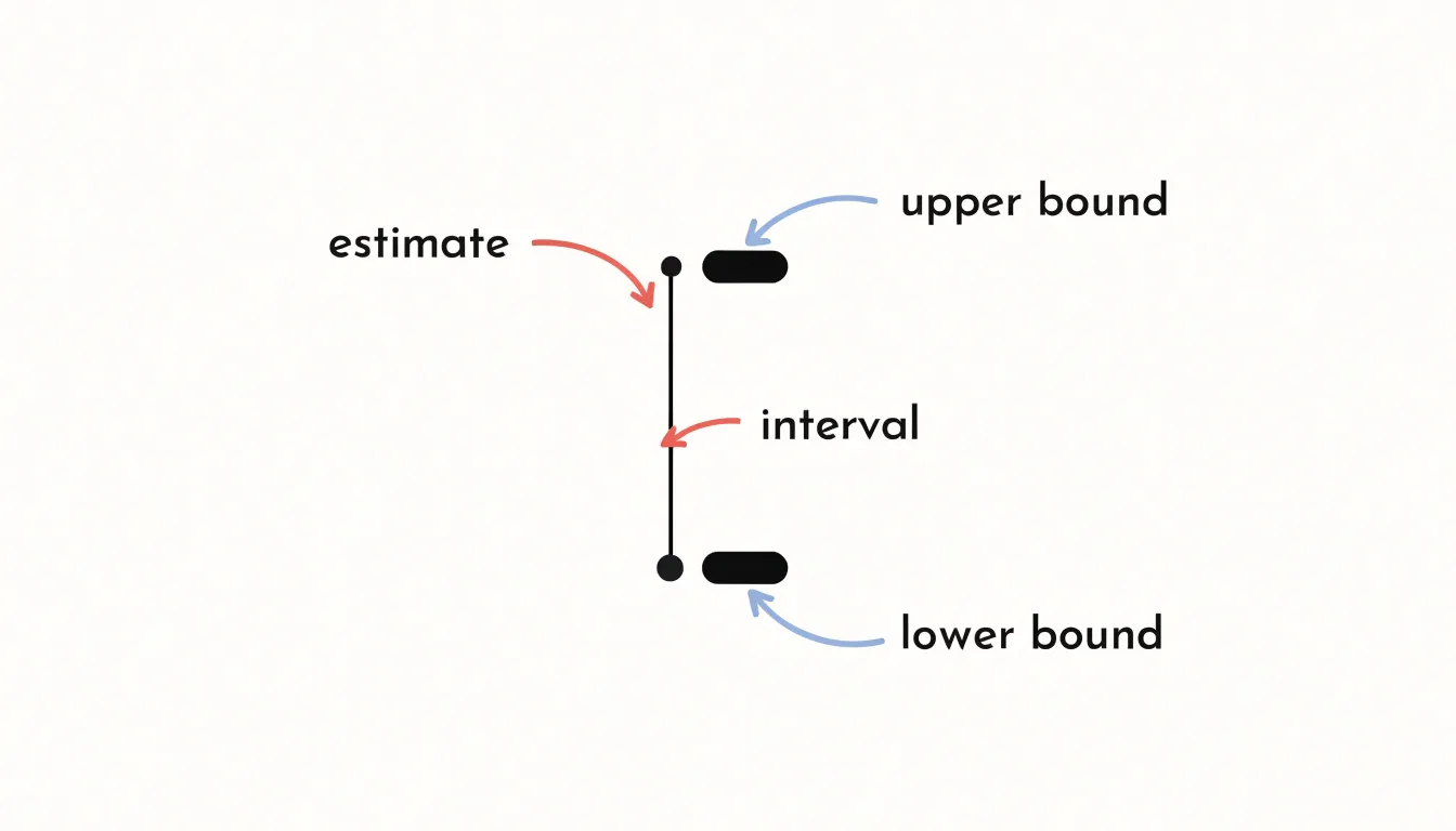
The vertical line maps a statistical range directly onto the chart’s coordinate system. If the y-axis measures a mean response, the segment from the lower cap to the upper cap spans the plausible range for that mean—whether derived from a standard deviation, a standard error, or a confidence interval. The caps serve as deliberate visual anchors: they close off the line so the eye registers a definite endpoint rather than a fading stroke, making it easy to compare the extent of one interval against another across the plot.
Horizontal error bars work the same way along the x-axis, and some charts carry both orientations at once, producing a cross of intervals around each point. The length of the bar encodes uncertainty: a long bar signals a wide range, a short bar a narrow one. Because the bars are drawn directly at the data points, the reader can see at a glance how precision varies across the series, where intervals overlap, and which estimates stand apart from their neighbors. The geometry is simple, yet it ties every plotted value to an explicit statement about how much confidence that value deserves.
Standard Deviation
Standard deviation describes how spread out your data is by summarizing the typical distance between individual data points and the mean of a single dataset. Collected measurements rarely cluster tightly at the average; some fall slightly above or below, and a few sit far away in either direction. Standard deviation turns this natural dispersion into a single number, showing whether observations are consistently close to the mean or widely scattered around it.
The calculation starts with the mean, the arithmetic average of all the values. Each data point’s distance from the mean—its deviation—is squared so positive and negative distances do not cancel out. Those squared deviations are averaged, and the square root is taken to return the result to the original units of the data. When the values come from a sample rather than a full population, the averaging step divides by one fewer than the number of observations ($n - 1$), an adjustment that corrects for a sample’s tendency to underestimate the spread of the wider population. Because the final figure is expressed in the same units as your measurements, it is directly interpretable.
A small standard deviation indicates that data points sit close to the mean, reflecting a tight, consistent dataset. A large standard deviation signals that values vary considerably across a wide range. In a lab setting, a small standard deviation across repeated measurements suggests a precise instrument and a stable procedure, while a large one points to variability that deserves investigation. Standard deviation thus serves as a fundamental descriptive statistic, capturing the natural spread within the data you actually have before any comparison to other estimates is made.
Standard Error
The standard error measures how much trust should be placed in a sample mean as an estimate of the population mean. When researchers draw a sample, the resulting average is just one value from a distribution of possible averages. Repeat the sampling process with new random draws, and the mean will land somewhere slightly different each time. The standard error quantifies this variability, measuring how precisely the sample average pins down the true population value. It is calculated by dividing the sample standard deviation by the square root of the sample size.
This construction gives the standard error a distinct role compared with the raw spread of the data. While standard deviation describes how widely individual observations scatter around their own mean, the standard error describes how widely the means of repeated samples would scatter. It is a statement about the accuracy of an estimate. A wide spread in the underlying measurements can coexist with a highly precise average, provided the sample is large enough.
Because the square root of the sample size ($n$) appears in the denominator, the standard error shrinks as the sample grows, but at a decelerating rate. Quadrupling the sample size halves the standard error; gaining another factor of two in precision requires four times the observations again. This diminishing return is a practical consideration in study design, since it sets expectations about what additional data collection can achieve.
In reporting, the standard error feeds directly into confidence intervals and significance tests, converting a point estimate into a statement of uncertainty. It offers a compact summary of how much a result might shift from sample to sample, helping readers judge whether an observed average is stable or merely an artifact of the particular observations collected.
Confidence Intervals
A confidence interval gives a range of plausible values for the true population mean, built from the sample data at hand. Because different samples drawn from the same population produce slightly different means, the confidence interval translates that sampling variability into a range around the estimate, expressing where the true population mean is likely to sit.
A 95% confidence interval is constructed so that, if the same sampling procedure were repeated many times, about 95% of the resulting intervals would contain the true population mean. This is a statement about the long-run behavior of the method. In practice, the interval is computed from the sample mean plus and minus a margin of error, which combines a critical value from the relevant distribution (often approximately 1.96 for a 95% level in large samples) with the standard error of the mean.
Because the standard error shrinks as sample size grows, larger samples yield narrower intervals and a tighter bound on the location of the true mean. The width also depends on the variability of the underlying data and on the chosen confidence level: a 99% interval is wider than a 95% one because it must capture the true value more often. These properties make confidence intervals a compact way to communicate both an estimate and its precision, allowing readers to compare results across studies on a common footing.
Range Bars
Range bars capture the full sweep of a dataset by marking its highest and lowest observed values. The top of the bar sits at the maximum, the bottom at the minimum, and the distance between them is the range itself. Each endpoint corresponds to a value that actually appeared in the sample, with no averaging, smoothing, or model fitting applied.
Because the endpoints are literal minimum and maximum values, range bars are sensitive to everything in the dataset, including a single outlier. One unusually large or small observation will pull the corresponding end of the bar outward and expand the apparent spread, making the graphic an honest but impressionable summary. This property is useful when the question of interest concerns the extremes—such as the hottest day in a season, the slowest response time in a trial, or the widest variation in a manufacturing batch.
Computing the endpoints requires only a scan for the smallest and largest entries, so range bars can be drawn quickly even for large datasets, and the resulting picture is easy to interpret without statistical training. Overlapping range bars show at a glance which groups share territory and which occupy distinct regions of the measurement scale.
Range bars work best alongside other summaries, since the endpoints say nothing about how observations distribute themselves in between. A dataset clustered tightly near its middle looks identical in range-bar form to one spread evenly across the same interval. Pairing the range with a measure of central tendency or an indication of density gives readers both the full extent of the data and a sense of its internal structure.
Overlapping Error Bars
When two groups are plotted side by side with error bars, a common rule of thumb is to check whether the bars overlap to judge if the difference between them is meaningful. If the bars overlap substantially, the two groups are often treated as statistically indistinguishable; if they are clearly separated, the difference is taken as likely real. Because each bar represents a range of plausible values around the group estimate, shared territory suggests the observed separation may be little more than sampling noise. The practical appeal is obvious: no formal test is required, and the comparison can be made at a glance.
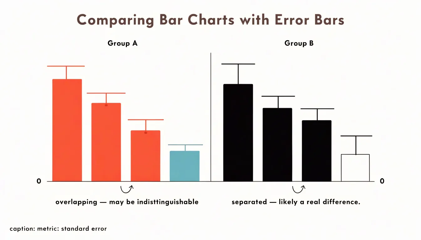
However, this heuristic has important limits. The width of an error bar depends on whether it represents a standard error, a confidence interval, or a standard deviation, and these metrics are not interchangeable. Two groups whose standard-error bars just touch may still differ significantly, because the standard error of the difference between means incorporates the variability of both groups and is larger than either alone. Conversely, bars that overlap by a small amount do not guarantee that a formal test would fail to find a difference. Overlap is therefore a screening aid rather than a verdict, and the specific metric used should be stated wherever such plots appear.
Treat visual overlap as a first pass. Clear separation invites closer scrutiny and a proper significance test; obvious overlap suggests the groups are close enough that any difference is likely small relative to noise. When the decision matters, compute the test directly rather than relying on visual impression, and report the interval alongside the p-value so readers can judge the size and uncertainty of the effect for themselves.
Bar Graphs
When a bar graph carries error bars, the reader faces two visual tasks at once: judging the height of each bar and judging the size of the uncertainty attached to it. Best practice begins with a consistent baseline, since bars encode value through length measured from zero. A truncated axis distorts perceived differences between bars and makes uncertainty intervals harder to interpret. Keep the y-axis starting at zero unless there is a strong, stated reason otherwise, and label the axis clearly so the reader knows what the heights represent.
Make the error bars legible in their own right:
- Specify the metric: State in the caption or axis label whether the bars show standard deviation, standard error, or a confidence interval (and at what coverage), and specify the sample size behind each bar.
- Maintain visual clarity: Choose a cap width and line weight that remain visible at the rendered size, and use a consistent convention (such as symmetric intervals around the mean) across all bars so comparisons are fair.
- Include numerical summaries: Provide means and interval bounds alongside the graphic so readers can verify visual impressions when comparing bar heights and interval overlap.
- Reduce clutter: Order bars by value or by a meaningful grouping to reduce cognitive load, and avoid crowding the plot with too many categories, which compresses spacing and shrinks the visual footprint of each error bar.
Consider whether a bar graph is the right display. Pairing bars with error intervals works best when values are positive, categories are few, and the reader’s task is comparing level and precision together. Add a horizontal reference line or annotations where they help readers judge whether intervals cross a meaningful threshold.
Line Charts
Line charts are a natural fit for continuous time-series data, where a sequence of points joined by segments along a horizontal time axis tracks direction, pace, and turning points. When the quantities being tracked are estimates rather than exact counts, error bands or shaded regions around the line complete the picture.
A shaded band drawn around a trend line marks the range within which the underlying value is expected to fall at each point in time, given the uncertainty of the measurement or model behind it. The band widens where data are sparse, where variability between observations is high, or where forecasts extend beyond the observed record; it narrows where measurements are dense and consistent. Readers can therefore see uncertainty as a changing quantity across the timeline rather than a single figure attached to the series as a whole—a dynamic that a single confidence interval or an aggregate margin in a caption would flatten.
Shaded regions also support comparison. Two trend lines with overlapping bands invite a cautious reading of differences, while clearly separated bands suggest a distinction worth noting. In forecast charts, the familiar cone shape communicates increasing doubt as projections reach further into the future, with the band’s boundaries showing plausible highs and lows at each horizon. A light, semi-transparent fill keeps the central line legible and lets gridlines show through, so the band informs the trend without obscuring it.
Scatter Plots
A scatter plot places individual data points across two dimensions, positioning each marker according to its X and Y values. When those values carry uncertainty, a bare dot conveys a misleading impression of precision. Adding two-dimensional error bars resolves this by extending horizontal and vertical lines outward from the point, capturing the range of plausible values along both axes at once. Physical sciences rely heavily on this convention: an astronomy paper plotting stellar magnitudes against temperatures will show a cross through each star, one arm spanning brightness uncertainty and the other temperature uncertainty, showing at a glance which points are tightly constrained and which are fuzzy.
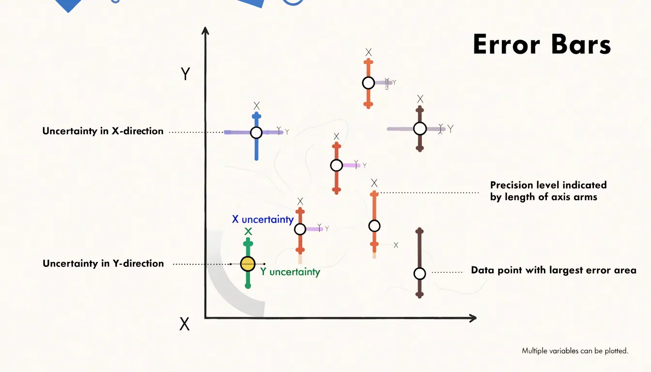
The horizontal segment runs from the low to the high bound of the X uncertainty, while the vertical segment does the same for the Y uncertainty, typically centered on the measured value. Symmetric bars use a single uncertainty magnitude in each direction, while asymmetric bars allow separate lower and upper bounds—which matters when a measurement is bounded below by zero or when confidence intervals are skewed. The two segments usually cross at the marker itself, though some styles offset the bars or cap their ends with short perpendicular ticks to make the bounds unmistakable.
These crosses let viewers perform an informal visual inference: points whose error bars fail to overlap along an axis are plausibly distinct in that dimension, while heavily overlapping bars suggest differences within the noise. By encoding uncertainty directly onto every marker, 2D error bars turn a scatter plot from a picture of point estimates into an honest portrait of what the data can and cannot support.
Common Mistakes
A recurring mistake in reading charts with error bars is treating bar length as a direct verdict on statistical significance. Readers often view a short error bar as proof that a result is meaningful, while dismissing a tall bar as noise. While a narrow interval does indicate a precise estimate, precision and significance are separate quantities, and conflating them leads to conclusions the underlying data cannot support.
A short error bar tells you only about the tightness of an estimate, not whether it differs meaningfully from a comparison value. A very precise measurement of a difference that is essentially zero will produce a short bar and no practical importance whatsoever. Conversely, a study with genuinely large effects but small samples or noisy measurements can produce tall bars even when the finding matters. Judging significance from bar length alone ignores the reference point, the effect size, and the number of observations behind the estimate.
Similarly, relying on visual overlap between two bars is a flawed shortcut, since a proper test uses the standard error of the difference rather than separate visual intervals. These misreadings compound when charts lack labels or captions explaining what the bars show, leaving readers to assume that short means real and tall means dubious. The practical remedy is to ask what quantity the bar represents, how many observations underlie it, and what comparison the claim requires, rather than letting visual length stand in for statistical reasoning.
Sample Size
Increasing the sample size is one of the most direct ways to shrink the error bars on a chart, due to how standard error is calculated. Because the standard error divides the sample standard deviation by the square root of the number of observations, the numerator (the spread of individual values) stays roughly fixed as long as the underlying population is stable, while the denominator grows with every additional observation. A sample of four cuts the standard error in half compared with a single observation; a sample of 16 cuts it to a quarter; a sample of 100 brings it to one-tenth.
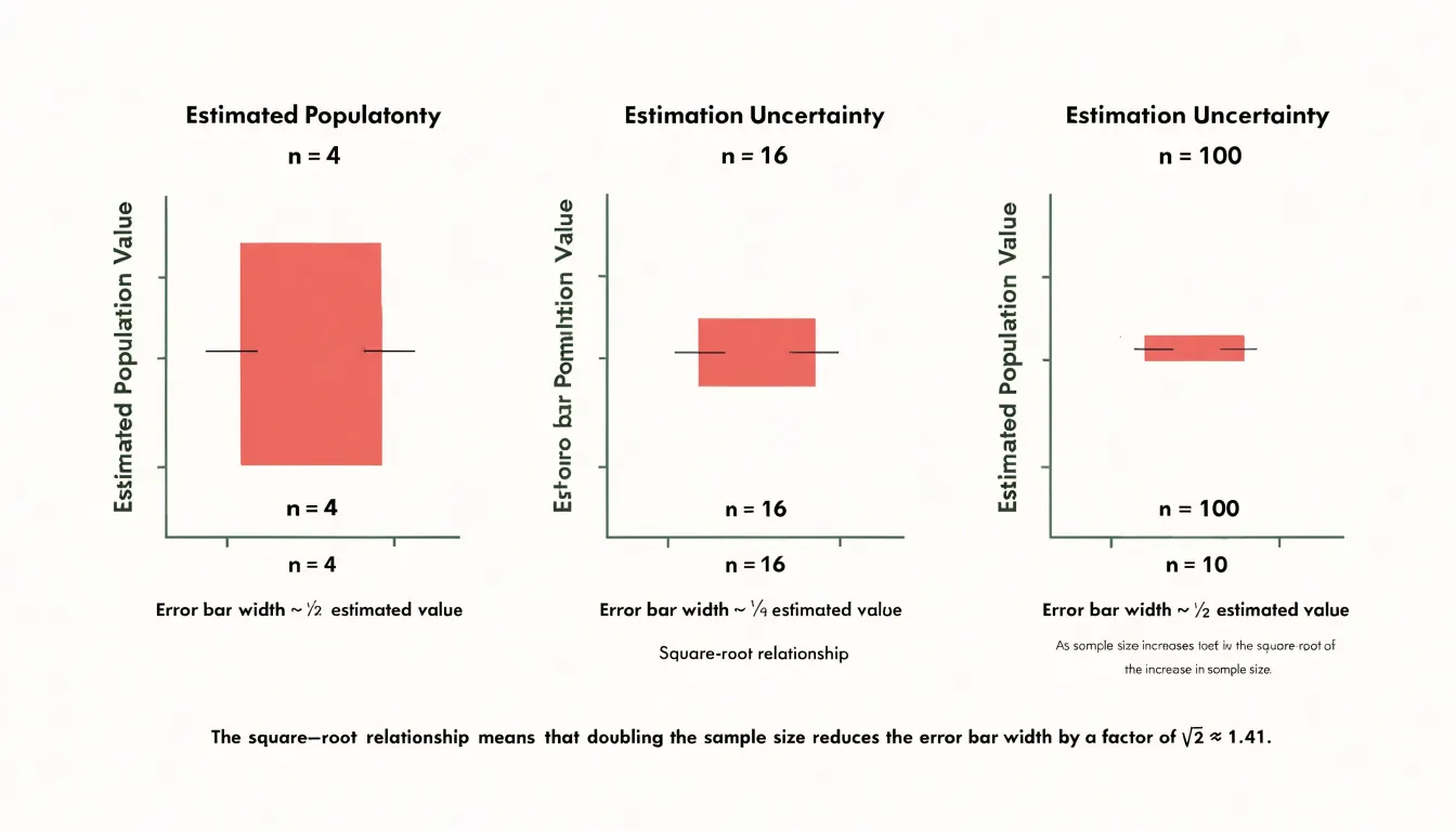
Error bars representing standard error or confidence intervals inherit this scaling directly. If the bars represent one standard error in each direction, doubling the sample size multiplies their length by roughly 0.707, and quadrupling the sample size halves them. This square-root relationship explains why early gains from collecting data feel dramatic and later gains feel marginal: going from 10 to 40 observations visibly tightens the bars, while going from 1,000 to 4,000 produces a smaller visual change for the same proportional effort.
This scaling also explains why very large samples can produce error bars so narrow they appear almost invisible, collapsing onto the estimate itself. That collapse reflects genuine statistical precision, though readers should remember that narrow bars describe the precision of the estimate rather than the spread of the underlying data, and that systematic bias in data collection does not shrink simply because the sample grows.
Real World Examples
The way error bars are drawn and explained in news graphics shapes how audiences understand uncertainty across different fields:
- Political polling: Election-season graphics often show a trend line with a shaded band or capped vertical bars representing the margin of sampling error. Case studies show that some outlets label the band clearly and note that overlapping intervals mean a lead may not be statistically meaningful, while others present a single line with no interval at all, inviting readers to treat small movements as real shifts in opinion.
- Climate reporting: Graphics summarizing temperature projections or emissions scenarios frequently display ranges derived from multiple model runs, using shaded envelopes or whisker plots to show the spread across simulations. While the width of the band carries the central message about uncertainty, captions sometimes omit what the range represents, leaving readers to guess whether it reflects model disagreement, natural variability, or observational error.
- Medical studies: News graphics reporting treatment effects often include confidence intervals on risk ratios or survival curves. Visual treatment varies widely, from clearly annotated forest plots to simplified bar charts where the interval is nearly invisible.
Across all three domains, error bars communicate uncertainty effectively only when the graphic, the caption, and the surrounding text work together to explain what the interval means and how it should influence interpretation.
Uncertainty Myths
One of the most persistent misconceptions about error bars is that they mark something gone wrong—that a visible error bar indicates a flawed measurement, and a wide bar signals a sloppy laboratory, an incompetent researcher, or a botched procedure. This framing treats uncertainty as a stain on the data rather than an honest description of it, leading students and the public alike to distrust precisely the results reported most carefully.
Every instrument has finite resolution, every protocol has limits, and every sample is drawn from a larger, unmeasured population. These sources of variability are the normal conditions of empirical work. A scientist who reports an error bar is not confessing to a mistake, but stating quantitatively how much the result could reasonably differ from the true value given the available tools and conditions.
Error bars capture distinct kinds of variation:
- Random fluctuation: Trial-to-trial variation that no amount of care can eliminate entirely.
- Systematic effects: Factors that shift all measurements in a consistent direction.
- Natural spread: Genuine diversity within the phenomenon itself, such as variation among biological specimens.
Stigmatizing uncertainty carries a practical cost: researchers face pressure to omit error bars, making results appear more definitive than the evidence supports. A field that hides its error bars is not more rigorous; it is simply less transparent. Precision and certainty are different things, and error bars exist to keep that difference visible.
Quick Reading Tips
Before drawing conclusions from a chart, run through three quick checks to guard against common misreadings:
- Check the axis scales: Note where each axis begins and ends and whether intervals are uniform, as a truncated vertical axis can make small differences look dramatic. Verify that both axes carry descriptive labels, clear units, and aligned gridlines, and check whether a transformation such as a logarithmic scale has been applied.
- Examine the error bars: Check the figure caption and legend for an explicit definition of what the bars represent (standard deviation, standard error, confidence intervals, or full data ranges). Notice whether the bars are symmetric or asymmetric, whether they extend in one direction or both, and whether they appear on every point or only on selected ones.
- Read the legend and metadata: Match each color, shape, line style, and marker to its category. Confirm the sample size behind each series, check whether categories are grouped in ways that could obscure differences, and locate the source and date of the data.
Final Takeaways
Fluency with error bars turns passive chart viewing into critical analysis. By checking what an interval represents, how it was calculated, and how many observations sit behind it, you can separate precise estimates from noisy ones and avoid mistaking visual overlap or bar length for a formal significance test. Recognizing uncertainty as an inherent part of measurement—rather than a flaw—helps you spot misleading graphics that omit intervals and evaluate claims in scientific literature, news reports, and business presentations based on the true reliability of the evidence.
Frequently Asked Questions
What do error bars show on a graph?
Error bars attach a visible measure of uncertainty to a plotted data point. The central marker sits at the estimated value, while the caps mark the boundaries of the interval the analyst wants to communicate.
What is the difference between standard deviation and standard error?
Standard deviation summarizes how spread out individual data points are around the mean of a single dataset. Standard error measures how precisely a sample mean estimates the population mean by describing how widely the means of repeated samples would scatter.
What does a 95% confidence interval mean?
A 95% confidence interval is constructed so that, if the same sampling procedure were repeated many times, about 95% of the resulting intervals would contain the true population mean. It is computed from the sample mean plus and minus a margin of error.
Can you tell if two groups are significantly different by whether their error bars overlap?
Overlap is a screening aid rather than a verdict. Two groups whose standard-error bars just touch may still differ significantly, and when the decision matters, a proper significance test should be computed directly.
How does sample size affect error bars?
Because standard error divides the sample standard deviation by the square root of the sample size, error bars representing standard error or confidence intervals shrink as the sample grows. Quadrupling the sample size halves the standard error, though the gains decelerate as sample size increases.
What should I check before interpreting a chart with error bars?
Check the axis scales, examine the error bars, and read the legend and metadata. Specifically, confirm what the bars represent, note whether they are symmetric or asymmetric, and verify the sample size behind each series.
Tony Astor
Tony writes about data visualization and the tools people use to build charts and dashboards. More about Data Illustrator