Dot Plot vs Bar Chart: Differences and Best Uses
 By Tony Astor ·

Dot Plot vs Bar Chart
A dot plot displays every individual data point as a dot along a single axis, stacking repeated values to show frequency, which preserves distribution shape, clusters, gaps, and outliers. A bar chart aggregates data into bars whose lengths represent totals or means per category, making it better for comparing group totals and handling large datasets.
Table of Contents
Dot Plot
A dot plot maps every single data point along a single axis, typically horizontal. Each observation is represented by a dot placed at its corresponding value on the axis. When multiple data points share the same value, dots are stacked vertically, creating a column that shows the frequency of that value.
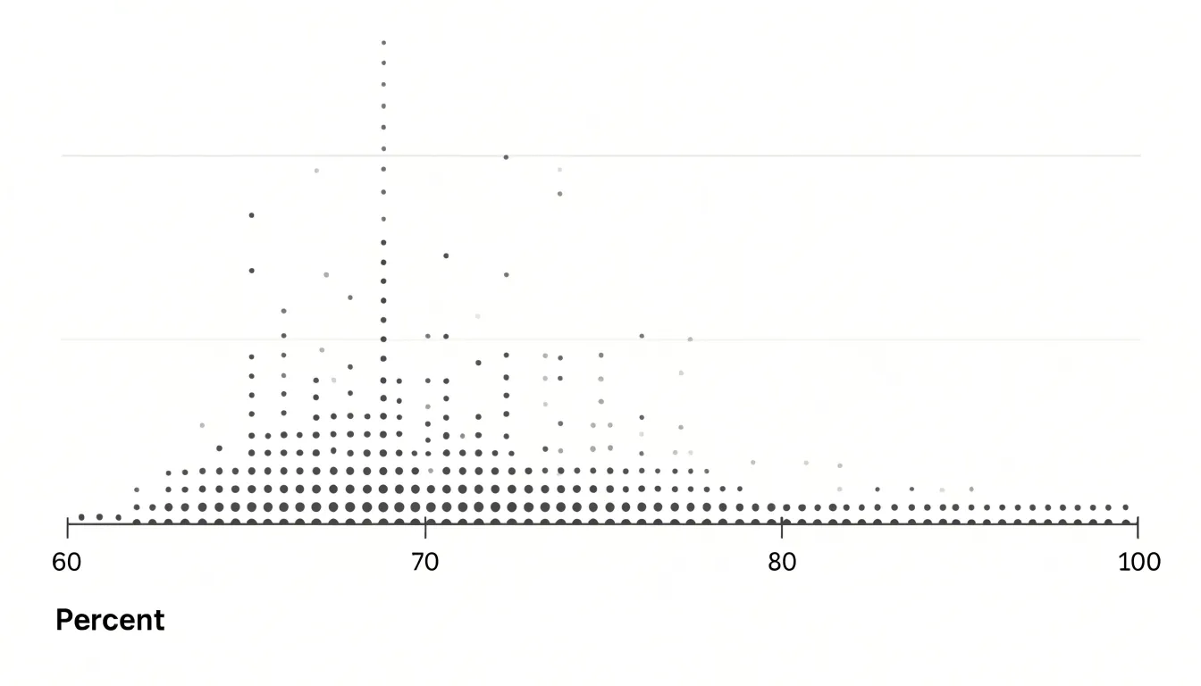
This one-to-one mapping preserves the granular details of the dataset, allowing viewers to see the exact distribution of values, identify clusters, gaps, and outliers, and understand the spread of the data without any loss of information. Unlike summary statistics or aggregated charts, a dot plot does not obscure the raw data; it presents it in a compact and intuitive form. The stacking of dots provides a clear visual sense of density, making it easy to compare frequencies across different values.
Dot plots are particularly effective when the dataset is small enough that individual points are distinguishable, typically up to around 20 or 30 observations. They are also useful for comparing distributions across groups by using separate dot plots or different colors. Overall, the dot plot excels at preserving the integrity of each data point while offering a clear view of the overall pattern, making it an essential tool for exploratory data analysis.
Bar Chart
A bar chart reduces a dataset to a set of discrete bars, one for each category, where the length of each bar represents a summarized total or aggregate value. Rather than asking a viewer to mentally tally dozens of individual records, the bar chart performs that aggregation in advance and encodes the result as a single visual length. When the goal is to compare totals across categories, this design removes friction: the eye simply scans the bars and ranks them by length, a judgment people make quickly and with high accuracy.
Because each category occupies its own clearly separated bar, there is no ambiguity about where one group ends and another begins. The bars can be ordered by value, by a natural category sequence, or alphabetically, giving the author control over how easily the ranking is perceived. Common variants extend this logic: horizontal bars accommodate long category labels without rotation, grouped bars place several totals side by side for subcategory breakdowns, and stacked bars show how a total decomposes into parts. In every case, position along a common baseline plus length encodes magnitude, and color or grouping distinguishes categories.
This makes bar charts especially effective for business reporting, survey results, and any situation where stakeholders need a clear read on which categories are largest, smallest, or roughly equal. The chart type also scales gracefully, handling a handful of categories or a few dozen without losing clarity, provided labels remain legible.
Small Data Sets
Dot plots work well with small data sets because every individual observation remains visible and can be traced back to its source, confirming that nothing has been merged, grouped, or smoothed away. A bar chart built from the same values summarizes counts into categories, so the individual identity of each observation disappears into a single bar height. With small samples, that loss of detail can matter considerably, since each data point carries weight in the overall picture and a single unusual value can influence averages and conclusions.
Dot plots also handle small samples without imposing arbitrary bins or intervals. The number line spans the observed range, and dots sit at their exact values, so no information is approximated. Grading scales, satisfaction ratings, counts of events per day, and similar discrete measures map naturally onto dots, and the resulting plot often needs no additional labeling beyond axis values. For small data sets, the dot plot gives an honest, complete rendering of the data while remaining quick to read and easy to construct by hand.
Large Data Sets
When a data set grows into the thousands or millions of observations, the marks on a dot plot begin to collide. Points that fall on the same or similar values stack up and overlap, turning the chart into a dense cloud where individual observations can no longer be distinguished. Increasing marker size only worsens the crowding, and reducing it makes overlapping even harder to read. Once the dots merge into a solid mass, the reader loses the ability to compare frequencies with any precision.
Bar charts handle heavy data volume by summarizing the data into counts, means, totals, or other statistics. The chart stays legible no matter how many underlying records feed into it, because visual complexity is tied to the number of categories rather than the number of observations. Ten thousand rows describing five categories still produce five clean bars, with heights that can be sorted for easy comparison and labels that remain readable.
This aggregation makes bar charts well suited to reporting workflows. Data can be grouped and summarized before plotting, conveying the essential pattern without the visual noise of raw points.
Clusters and Outliers
Dot plots reveal the shape of a dataset through the arrangement of individual points:
- Clusters appear as dense stacks or groups of dots where many values fall close together, such as a common range of test scores or typical daily temperatures. Identifying a cluster helps you spot where the majority of observations lie, revealing central tendencies without calculating averages.
- Gaps are empty spaces along the number line where no data points exist. A gap suggests a break in the data, perhaps indicating a natural threshold or a missing category. In a dot plot of customer ages, for instance, a gap might separate younger and older demographics, prompting further investigation.
- Outliers are individual points that sit far away from the rest of the data, often isolated on either end of the plot. Because extreme values can skew statistical measures like the mean, spotting them visually is a quick way to assess data quality or uncover unusual cases.
By examining clusters, gaps, and outliers together, you gain an immediate sense of the distribution’s spread, symmetry, and potential anomalies without formulas or software. You can also compare multiple dot plots side by side to see how clusters shift or outliers emerge across different groups.
Group Totals
Bar charts excel at summarizing group totals, offering a natural starting point for readers who need orientation before examining finer detail. When each bar represents a category aggregate, the eye ranks the bars almost instantly, letting the overall structure of the data register before any numbers are consulted.
Averages follow the same logic. If each bar reflects the mean value for its group, differences in bar height translate directly into differences in average performance, spending, response time, or whatever quantity the chart encodes. Readers can identify high-performing and low-performing groups in a single sweep and judge whether the averages cluster tightly together or spread widely across the range.
Broad trends also emerge from the sequence of bar heights. When categories follow a meaningful order—such as time periods, regions ranked by size, or progressive stages—the profile of the bars reveals direction and shape. A steady climb, a plateau, a sharp peak, or a lopsided concentration all become visible without statistical training. This supports mixed audiences simultaneously: heights allow quick comparison, while labels and axis values provide precise confirmation.
Continuous Data
Continuous data presents challenges because values can fall anywhere along a range, and how a chart groups those values shapes what the viewer perceives. By placing each observation directly at its exact value on a number line, dot plots avoid forced binning.
When continuous values are divided into bins, the analyst must choose the number and width of those bins, and each choice alters the visual result: wide bins smooth away detail and can merge distinct clusters, while narrow bins scatter the data into a noisy, spiky pattern. Dot plots sidestep this trade-off. Each distinct value gets its own column of marks, preserving the genuine shape of the distribution—including its peaks, gaps, tails, symmetry, or skew—at a level of detail that grouped charts can obscure. For exploratory analysis of continuous measurements such as times, weights, or scores, this fidelity makes dot plots a dependable first view before any summarization takes place.
Categorical Data
Bar charts are built around separation: each category receives its own bar, with a visible gap of white space between neighbors. The eye reads these gaps as boundaries, instinctively treating every bar as a self-contained entity. When a dataset consists of labels such as product names, regions, departments, or survey responses, this visual separation mirrors the structure of the data itself.
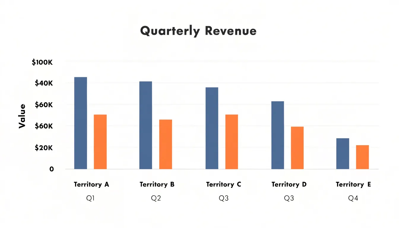
Sorting the bars from largest to smallest turns the chart into an ordered list with magnitudes attached. Audiences can see who leads, who trails, and how wide the gap is between adjacent ranks without consulting a table, making bar charts a natural fit for leaderboards and budget breakdowns.
Nominal data types—categories without any inherent order, such as colors, brands, or machine types—sit comfortably side by side in a bar chart because nothing about the layout implies sequence. Counts and frequencies map naturally onto bar length, communicating both the identity of each group and its relative size in a single view.
Building Charts
Constructing a dot plot begins with deciding on the categorical or numeric axis and determining how observations stack vertically. Manually, a person lists each category or value along the horizontal axis, marks a baseline, and places one dot for every observation, aligning repeated values carefully so columns stay tidy. Software automates this stacking through frequency counts or binning; most plotting libraries treat the dot plot as a variant of a strip or Cleveland dot chart, reducing the code to a few lines once the data are shaped properly. The main effort lies in ensuring that dot size and spacing preserve readability when counts grow.
Bar charts follow a different construction path because the builder must aggregate values before drawing. Manually, this means computing totals or means, setting a scale, and drawing rectangles to match. In software, the bar chart is a default template in nearly every tool, with automatic axes, labels, and color handling.
The trade-off appears in flexibility. A dot plot adapts easily to raw, unaggregated observations and to overlaying multiple groups because dots can be layered without occlusion. A bar chart organizes around pre-computed summaries, so changing the underlying statistic or adding a second grouping variable often requires rebuilding the aggregation step. That difference shapes the setup time, the number of steps, and the amount of intermediate data preparation each method demands.
Bar Chart Layouts
Bar charts can be drawn in two basic orientations: vertical column charts place categories along the horizontal axis with bars rising upward, while horizontal bar charts place categories along the vertical axis with bars extending to the right. Both encode the same quantitative information, so the decision comes down to label fit and scanning ease.
Horizontal bar charts suit situations where category labels consist of multi-word phrases, full sentences, or names running to twenty or thirty characters. A vertical layout forces such labels to be rotated or truncated to avoid overlapping, and rotated text is slower to read. A horizontal layout gives every label a full line of space along the left edge, keeping text level and legible.
Traditional vertical column charts work well when labels are short, such as single words, abbreviations, years, or brief codes like “Q1” or “FY24.” Short labels sit comfortably beneath each column without colliding, and the vertical orientation benefits from the natural left-to-right reading order. Column charts are also often expected for time-based categories such as months or quarters, since progress along the horizontal axis mirrors the passage of time.
When weighing the two, count the characters in your longest label and consider how many categories you have. Long labels or many categories favor horizontal bars, while brief labels and a modest number of categories favor vertical columns.
Grouped and Stacked Bar Charts
Grouped and stacked bar charts extend the basic bar chart to handle more than one categorical dimension at once.
In a grouped bar chart, each primary category occupies a position along the axis, and within that position several bars sit side by side, one for each sub-category. This lets a reader compare values across sub-categories within a group and track how a given sub-category performs across groups. For example, sales figures broken down by region and product line can show regions on the axis and a cluster of product bars at each region, making both regional totals and product mix visible in a single view.
In a stacked bar chart, sub-category values are placed on top of one another so that each bar’s total height represents the combined value for that group. This design emphasizes part-to-whole relationships, showing how each sub-category contributes to the overall total and how that composition shifts across groups—such as the share of revenue coming from each channel across different quarters.
The choice between them depends on the question being asked:
- Grouped bars support direct comparison of individual sub-category values because each bar starts from the same baseline.
- Stacked bars support comparison of totals and composition, though comparing middle segments across groups is harder since only the bottom segment shares a common baseline.
Both forms demand care with color, legend placement, and segment ordering to remain readable.
Avoiding Clutter
Both dot plots and bar charts benefit from disciplined formatting that strips away anything the data does not need:
- Axis scales: A bar chart encodes value through length, so its value axis should begin at zero to avoid exaggerating differences between bars. A dot plot encodes position, which permits a truncated axis when the data cluster sits far from zero, provided the truncation is clearly labeled.
- Gridlines and borders: Keep gridlines light, thin, and few. In dot plots, a single set of faint horizontal reference lines often suffices; bar charts may need only a baseline and occasional tick marks. Remove vertical gridlines entirely unless they mark meaningful categories, and avoid boxed chart areas.
- Spacing: In dot plots, keep consistent vertical spacing between category rows so no row appears more important than another. If multiple series share a row, separate their dots with a small, uniform offset or use distinct shapes rather than relying on color alone. In bar charts, a common rule is a gap roughly half to two-thirds the bar width, which keeps bars from merging visually while avoiding a sparse, disconnected look.
- Dot sizing: Dots should be large enough to register clearly at typical viewing sizes but small enough not to overlap or crowd neighboring rows and columns. When dots represent counts or weights, scale area rather than diameter so viewers read magnitude correctly, and add a legend showing reference sizes. Keep sizing consistent across a series.
- Color and labels: Limit color to a small palette tied to meaning, label axes directly where possible, and remove redundant titles, borders, and tick marks.
Real World Examples
Consider two everyday situations where data structure guides chart choice.
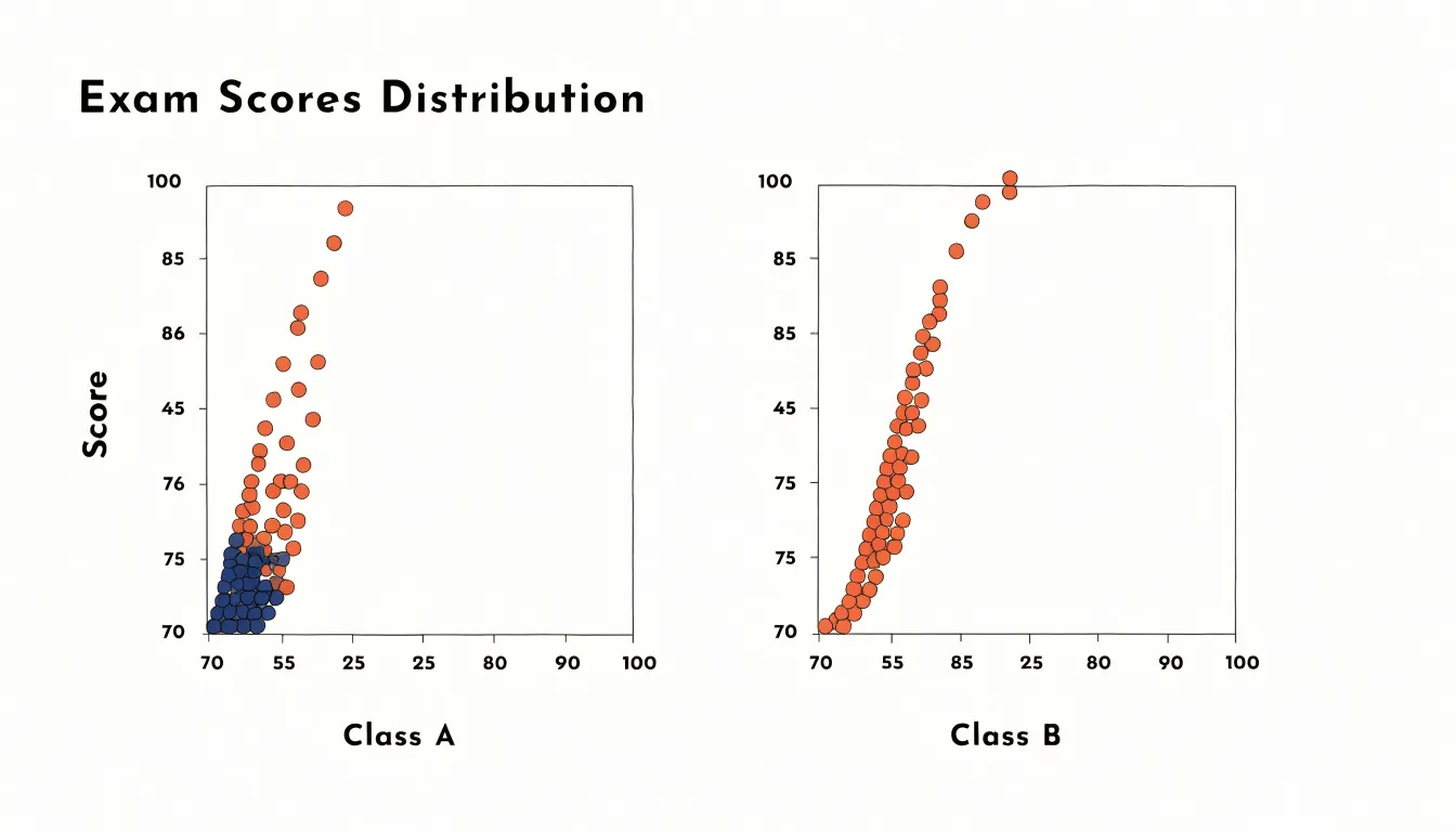
In a classroom, a teacher has just finished grading a unit exam for thirty students and wants to understand the shape of performance before deciding on the next lesson. Plotting each score on a dot plot reveals whether the class bunched around the middle, whether a few high achievers pulled ahead, or whether a small group lagged behind and needs targeted support. Individual values remain visible, so a score of 92 is not buried inside a bin. When the same exam is given to a second class, the teacher can compare the two dot plots side by side and spot shifts in the distribution at a glance.
In a regional sales office, a manager overseeing five territories wants to compare revenue across them for the most recent quarter. A bar chart assigns each territory a vertical bar whose height corresponds to total revenue, making it clear in seconds which region led, which trailed, and by how much. When the data spans several quarters, grouped bars allow side-by-side comparison of territories across time, revealing seasonal patterns and growth trends. The teacher studies distribution and spread at the individual level, while the manager compares aggregate totals across categories.
Key Differences
This quick-reference matrix summarizes the main differences across data type, dataset size, complexity, and primary visual goals:
- Data type: Dot plots are ideal for quantitative data plotted along a continuous scale where individual values are meaningful. Bar charts are suited for categorical data where bar length encodes a count or aggregate value.
- Dataset size: Dot plots handle small to moderate datasets effectively, whereas bar charts scale to large datasets by aggregating observations into categories.
- Complexity: Dot plots require minimal design elements and show raw data without transformation, aiding transparency. Bar charts involve more design choices—such as bar width, spacing, and color—and can become visually complex with many categories, though they remain familiar to most audiences.
- Primary visual goals: Dot plots show the distribution of individual values (clusters, gaps, and outliers) and compare distributions across groups. Bar charts compare aggregate values across categories, emphasizing rankings and differences in magnitude rather than distribution shape.
Choosing a Chart
A few simple questions can form a decision flowchart to guide your choice:
- What is the primary goal? To compare individual data points, reveal distribution patterns, or avoid the visual weight of bars, choose a dot plot. To compare summarized quantities and rankings across groups, choose a bar chart.
- What type of data do you have? Use bar charts for categorical data where each category has a single aggregate value, and dot plots for numerical data where you want to show distribution.
- How many data points are you displaying? For datasets with fewer than, say, 50 points, dot plots can be very effective. For larger datasets, use a bar chart or another summary visualization to avoid clutter.
- Who is the audience? Bar charts are widely understood and accessible for general audiences. Dot plots might require a bit more explanation but offer precision for analytical audiences.
Frequently Asked Questions
What is a dot plot used for?
A dot plot maps every individual data point along an axis and stacks dots when values repeat, preserving the exact distribution of values. It is useful for spotting clusters, gaps, and outliers while keeping each observation visible.
When should I use a bar chart instead of a dot plot?
Use a bar chart when comparing summarized totals, averages, rankings, or aggregate values across categories, especially with large datasets. Use a dot plot when you want to compare individual data points or show the distribution of numerical data.
How many data points can a dot plot handle?
Dot plots are particularly effective when the dataset is small enough that individual points are distinguishable, typically up to around 20 or 30 observations. With thousands or millions of observations, dots collide and overlap, making frequencies hard to compare.
How does a dot plot show clusters and outliers?
Clusters appear as dense stacks or groups of dots where many values fall close together, while gaps are empty spaces where no data points exist. Outliers are individual points far away from the rest, often isolated at either end, and can skew measures like the mean.
Should a bar chart axis start at zero?
Yes. Because a bar chart encodes value through length, its value axis should begin at zero to avoid exaggerating differences between bars. A dot plot encodes position, so it permits a truncated axis when the data cluster sits far from zero, provided the truncation is clearly labeled.
What is the difference between grouped and stacked bar charts?
Grouped bar charts place several sub-category bars side by side within each primary category, supporting direct comparison of individual sub-category values. Stacked bar charts place sub-category values on top of one another so each bar’s total height represents the combined value, emphasizing totals and part-to-whole composition.
Tony Astor
Tony writes about data visualization and the tools people use to build charts and dashboards. More about Data Illustrator