Dot Plot: Types, Uses and Examples
 By Tony Astor ·

Dot Plot
A dot plot is a graph where each observation is shown as one dot above a number line, with dots stacking vertically when values repeat. It preserves every individual data point, making frequencies, clusters, gaps, and outliers directly visible. It works best for small sets of discrete, counted data and supports accurate comparison by position along a shared scale.
Table of Contents
Dot Plot Basics
A dot plot is a graphical display in which each observation in a dataset is represented by a single dot placed above a number line. The dot’s position along the axis corresponds to the observation’s value, and when several observations share the same value, their dots stack vertically in a column. This one-dot-per-observation approach keeps every individual data point visible, allowing a reader to see the exact composition of the dataset at a glance rather than a summary of it. The result is a chart that functions as both a picture and an enumeration of the data.
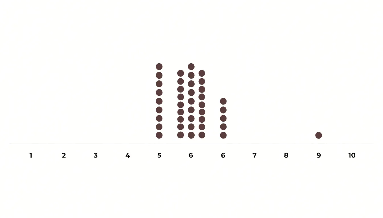
Dot plots work best with small sets of counted, discrete data. With a few dozen values, the columns stay short enough for individual dots to be distinguished and counted. Discrete data—such as the number of pets per household or goals scored in a match—fits naturally because the values fall on distinct points along the axis, making the plot especially suited to whole-number counts that cannot be split into fractions.
The chief strength of the dot plot is that it preserves the identity of each data point. Unlike a bar chart or histogram that groups values into bins, a dot plot never obscures how many observations took a particular value or how they are distributed. A reader can count the dots in a column to learn that value’s frequency, spot gaps where no data occur, and identify the smallest and largest values directly from the ends of the distribution. Clusters, outliers, and the overall shape of the data all remain visible, offering a compact, transparent view for small datasets where exact counting matters.
Chart Elements
A dot plot is built around three structural components:
- Horizontal axis: Serves as the measuring line for the variable under study. Values are marked at regular intervals, and the scale determines how precisely each observation can be placed. Clear tick marks and labels let readers identify each dot’s position without ambiguity. For categorical data, the axis functions as a series of labeled slots, one for each category.
- Category or value labels: Sit beneath the axis to identify what each position represents, whether a numerical value or a distinct group. Clear, evenly spaced labels ensure each stack of dots is associated with the correct value. For numerical data, labels typically appear at regular intervals rather than at every possible value, keeping the chart uncluttered while allowing accurate reading.
- Vertically stacked dots: Carry the frequency information. Because each dot sits above its matching axis value, the height of each vertical column encodes frequency: a tall column indicates a value that occurred many times, while a single dot indicates a value that appeared once. Reading across the axis and comparing stack heights gives a direct visual sense of the distribution’s shape.
Dot Plots vs Bar Graphs
Dot plots and bar graphs both display quantitative values across categories, yet they produce very different visual impressions. A traditional bar chart represents each value with a filled rectangle whose height or length encodes magnitude. Because those bars carry substantial visual weight, a chart with many categories quickly becomes crowded, drawing the viewer’s eye to the mass of ink rather than the numbers. A dot plot replaces each bar with a compact marker along a shared axis. Removing the solid fill strips away graphic material, so the same values occupy less space and avoid the overlapping labels and heavy shading common in dense bar charts.
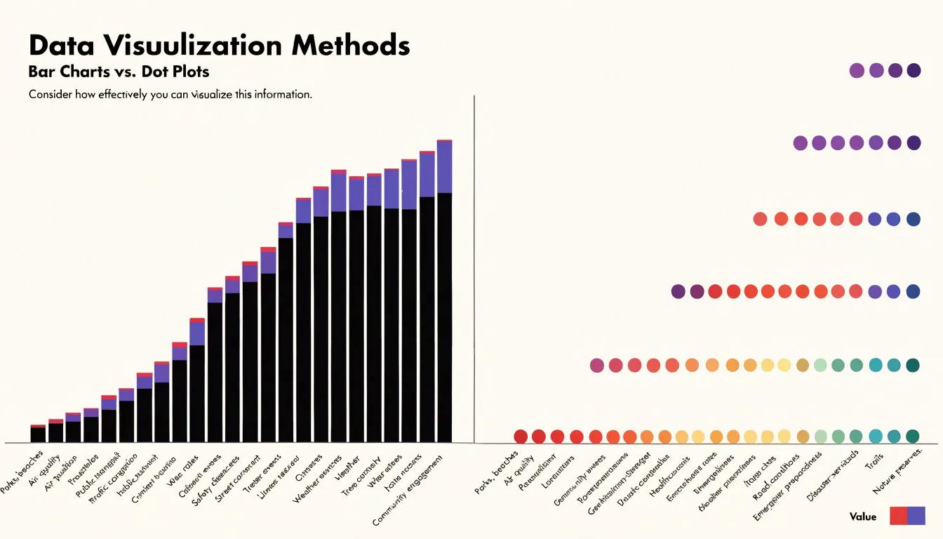
Data density follows from the same design choice. Dot plots can pack many categories into a narrow panel because each observation requires only a small symbol, and the absence of bar width means categories can be spaced closely without merging into a solid block. This makes dot plots well suited to ranked lists, long category inventories, and comparisons across groups on a shared scale.
The clearest distinction concerns how individual values are perceived. A bar chart emphasises the overall area of each rectangle, making small differences between adjacent bars difficult to judge. In a dot plot, each value is marked by a discrete point at an exact position, so the reader can compare positions directly against gridlines or a reference line. Outliers and unusually high or low values stand apart naturally, supporting precise reading rather than impressionistic comparison of filled shapes.
Simple Dot Plots
A simple dot plot displays counted values by placing one dot per observation above a discrete category or integer value on a single axis. Because every dot stands for one observation, a reader can count them directly rather than estimating from the length of a bar or the slope of a line, making the display easy to interpret even for audiences with little statistical training.
To construct the plot, data are organized by value or category, and each occurrence is placed above the appropriate axis position. As dots accumulate into vertical columns, the resulting silhouette gives an immediate impression of center, spread, and shape.
Minimal visual clutter is a defining strength of this format. There are no gridlines, legends, or shaded regions competing for attention, and no scales beyond the axis itself. The viewer’s eye moves directly from the axis positions to the stacks of dots, so patterns such as a single peak, two distinct clusters, or a long tail emerge without effort.
Wilkinson Dot Plots
Leland Wilkinson introduced a technique that adapts the dot plot to continuous quantitative data by first binning the variable into discrete intervals and then stacking a dot for each observation that falls within a bin. The procedure divides the data range into equal-width bins, counts how many values land in each one, and places that many dots in a vertical column centered on the bin’s position along the horizontal axis. What emerges is a histogram-like silhouette built from individual marks rather than solid bars, keeping every observation visible.
The choice of bin width governs the appearance of the result. Narrow bins spread the dots thinly and can reveal fine structure such as gaps or slight skew, while wider bins aggregate more observations into taller stacks and smooth away small irregularities. Because the dots carry no aggregation beyond their count, the reader can mentally reconstruct the data at any level of detail the bin width permits, and analysts often try several widths to balance clarity against fidelity to the distribution’s shape.
Stacking also solves the overplotting that afflicts naive dot plots of continuous variables, where many points at nearly identical values collapse into an unreadable smear. Assigning each observation to a bin and stacking symmetrically about the bin center keeps every point distinct and avoids the misleading impression of a trend that a one-sided stack might create. Uniform bin spacing along the axis ensures that chart distances correspond to data distances, preserving proportional relationships.
Cleveland Dot Plots
The Cleveland dot plot emerges from William Cleveland’s investigations into graphical perception at Bell Labs during the 1980s alongside collaborators like Robert McGill. Their experiments tested how accurately readers decode quantitative information from different visual encodings. A central finding was that position along a common scale—as in a simple dot or scatter plot—supports more accurate judgments than length, angle, area, or the varying bar lengths of a conventional bar chart. Cleveland’s dot plot applies this principle directly: each category receives a thin horizontal baseline, and a single dot marks its value along a shared numerical axis. The result is a compact display that uses the visual language of a scatter plot while handling categorical groupings.
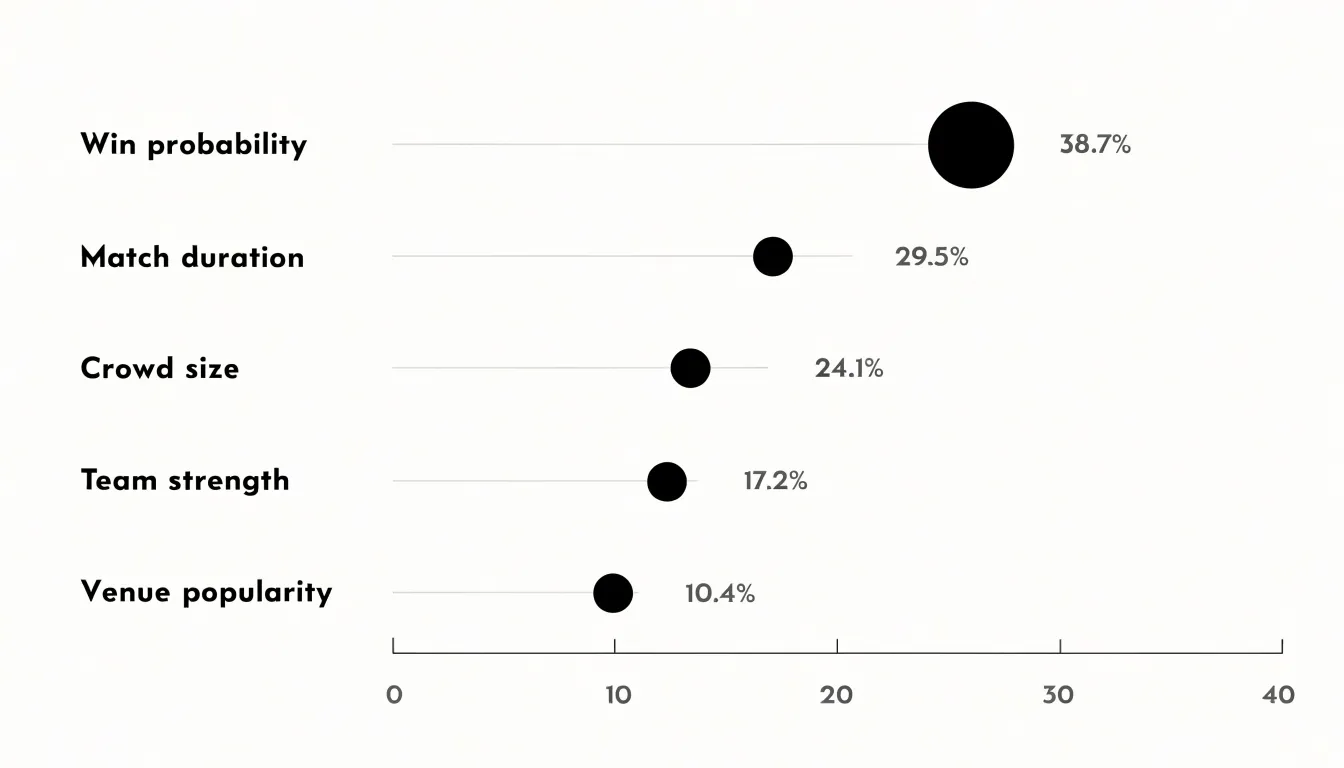
The horizontal orientation carries practical advantages. Long category labels sit comfortably at the left edge without the rotation or truncation common in vertical bar charts. Comparing dot positions rather than bar extents allows precise judgments across many categories while using ink sparingly. Sorting categories by value rather than alphabetically is a natural companion practice; once dots are ordered, trends, outliers, and clusters stand out immediately, and the sorted dot plot functions as an effective alternative to the pie chart for part-to-whole comparisons.
Cleveland documented the method in his 1985 book The Elements of Graphing Data and elaborated it in Visualizing Data (1993), where grouped and multi-panel variants appeared. Descendants include the dumbbell plot, which connects two dots per category to show change, and the lollipop chart, which pairs a dot with a thin stem. Software libraries in R, Python, and elsewhere offer dedicated dot plot functions, making the technique standard in exploratory data analysis and statistical reporting.
Paired Dot Plots
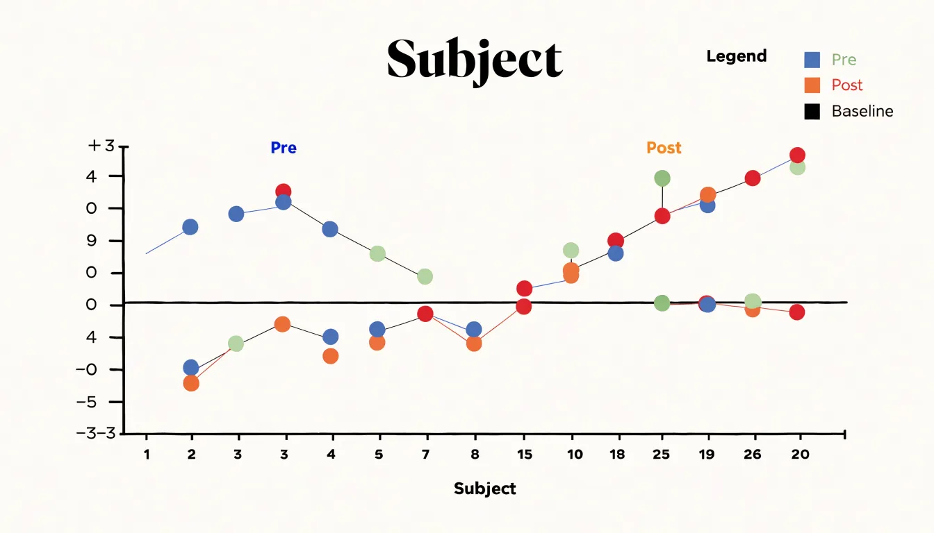
Paired dot plots compare two related datasets by placing both series on the same chart axis, allowing viewers to read differences directly against a shared scale. The most common arrangement aligns each pair of values vertically, so that pre-treatment and post-treatment results for the same subject sit one above the other at identical horizontal positions. Readers can scan down the chart to see whether the second value consistently rises above the first, falls below it, or scatters irregularly. Because the axis is shared, the distance between the two dots in each pair corresponds to the magnitude of change without requiring a separate table of differences.
Paired dot plots are widely used when the same units are measured twice—such as before and after an intervention, at two time points, or under two experimental conditions—or for dual metrics recorded on a common scale for the same entity, such as systolic and diastolic blood pressure or two test scores from the same candidate. Connecting the paired dots with a thin line emphasizes the within-pair relationship and helps the eye track each case across conditions. Consistent spacing between pairs, distinct markers or colors for the two series, a legend naming each condition, and a horizontal reference line for the baseline value keep the display legible and highlight the direction of change even when dozens of pairs are shown.
Finding Clusters and Outliers
In a dot plot, the spacing of marks along the axis carries most of the meaning. When dots stack in consecutive columns with little or no gap between them, they form a modal cluster. Taller columns signal values that recur often, and neighboring columns of similar height suggest a broader concentration zone where the bulk of the data lives. Tracing the silhouette from left to right shows where the mass gathers and where the field thins out. A long run of evenly spaced single dots marks a sparse stretch, and a gap interrupting an otherwise continuous run shows a shortage of values across a specific interval.
Outliers appear as isolated dots sitting well apart from the nearest cluster, often several empty units away. A quick visual scan can pick them out before any calculation is performed. Isolated marks near one edge can indicate a rare but genuine value, while a lone dot far from a tight central mound may warrant closer inspection as a possible recording error or an unusual case. Together, cluster recognition and outlier spotting give a fast overview of a dataset’s structure without arithmetic—revealing where typical values sit, whether the spread is symmetric or lopsided, and which observations deserve follow-up.
Measuring Spread
Measuring spread is essential for understanding the variability within a dataset. Analysts combine visual inspection with two primary numerical measures:
- Range: The difference between the maximum and minimum values. The range provides a quick sense of overall spread, but it is sensitive to outliers and does not capture how values are distributed between the extremes.
- Interquartile range (IQR): Focuses on the middle 50% of the data by subtracting the first quartile (25th percentile) from the third quartile (75th percentile). The IQR is more robust to outliers and offers a clearer picture of where the bulk of the data lies.
- Gap and cluster analysis: Examining the scale for regions with no data points, which can signal natural breaks, multimodal distributions, or separate populations within the dataset.
Combining range, IQR, and gap analysis assesses variability comprehensively. For instance, a wide range with a small IQR suggests outliers, while a large IQR indicates a more spread-out central portion. Visual tools like dot plots or box plots complement these numerical measures by displaying the spread and gaps graphically. In quality control, finance, and scientific research, these methods inform decisions about data reliability, the presence of anomalies, the causes of gaps, and the choice of robust summary statistics or statistical models.
Example
A classroom test score pattern illustrates how a dot plot works in a familiar setting. Suppose a teacher has recorded exam results for thirty students on a scale covering observed scores from 40 to 100. Rather than scanning a list of numbers, the teacher places a dot above the horizontal number line for each student’s result. A score of 75 earned by six students becomes a stack six dots high, while a score of 92 earned by one student appears as a lone dot.
Reading the finished plot reveals the class performance without calculation: the tallest stack marks the most common score, the spread shows how tightly results cluster, gaps expose scores nobody achieved, and isolated dots at the far ends highlight unusual performances. The teacher can use this view to judge whether the test was pitched at the right level, whether most students mastered the material, and whether a few outliers need attention. The same approach works for quizzes, homework, or any repeated measure collected across a group.
Example
Daily temperature tracking shows how a dot plot can reveal patterns over time. Suppose you record the high temperature each day for a month, yielding about thirty data points. Each day’s high becomes a dot placed above its date on the horizontal axis, while the vertical axis shows the temperature value.
The resulting sequence makes trends and anomalies apparent. A gradual increase from the beginning to the end of the month suggests a seasonal warming trend, while dots standing far above or below the typical range represent anomalous spikes—such as a heat wave or cold front. You can also split the month into weeks to see how the distribution shifts across periods. Because each dot represents a single day, the plot preserves daily granularity while providing a holistic view of the month’s weather, a combination equally useful for tracking daily sales or other time-series metrics.
Example
Customer wait time surveys generate duration measurements that are difficult to interpret from raw numbers or summary averages alone. Plotting each recorded service duration along a horizontal axis shows managers at retail counters, call centers, and clinic reception desks where most interactions fall, how wide the spread is, and whether a handful of unusually long waits are stretching the distribution.
In this context, the dot plot helps reveal operational bottlenecks. A large concentration of dots at a particular duration followed by a thin trail extending far to the right suggests that a subset of customers is experiencing delays that most others avoid. Managers can then investigate the processes, staffing levels, or time-of-day conditions associated with those longer waits. Similarly, peak queue lengths often correspond to visible humps where durations cluster around a higher value during busy periods.
Placing dot plots side by side also lets teams compare wait times across shifts, branch locations, or survey waves, turning routine surveys into an accessible diagnostic instrument for stakeholders without a statistical background.
Creating Dot Plots
Creating a dot plot by hand begins with preparing the axes:
- Draw a horizontal number line on grid paper, choose a scale covering the full range of your data, and label tick marks at regular, equal increments (such as one unit or ten) so spacing stays proportional.
- Write the variable name and relevant units beneath the line.
- Sort or scan your data and place a dot for each observation directly above its corresponding tick mark.
- When a value repeats, stack additional dots vertically at an equal distance from one another, leaving a small, consistent gap between adjacent columns so neighbouring stacks do not merge.
- Add a chart title and a brief note on the sample size.
Spreadsheet software automates this process. In Excel, first build a frequency table by listing each distinct value in one column and using COUNTIF in the next column to tally occurrences. Select both columns, insert a scatter chart, and format the series as solid circles with no connecting line. Adjust the axis minimum and maximum to frame the data tightly, remove distracting gridlines, and add axis titles. Google Sheets follows a similar path, using COUNTIF in a frequency table and a scatter chart with the line style set to none. Both tools let you resize markers, refine spacing, and export the finished chart as an image.
Formatting and Clarity
Deliberate choices about scale increments, spacing, and labeling determine how easily a reader can extract meaning from a dot plot:
- Scale increments: Select the smallest increment that keeps distinct data values visibly separate, then round to a familiar unit such as 1, 2, 5, 10, or 25 so mental arithmetic stays easy. Too fine a step produces a crowded axis; too coarse a step compresses meaningful differences into a single position. Keep tick marks uniform and extend the scale slightly beyond the minimum and maximum values so no dot sits flush against the chart border.
- Dot sizing and stacking: When many observations share a value, cap the stack height or allow a small horizontal offset so clusters remain legible without suggesting extra values. Keep dot diameter consistent across horizontal dot plots, since varied sizes distort perceived frequency.
- Labeling and whitespace: Place the axis title and units in a consistent position, keep number labels horizontal rather than rotated where space permits, and use a readable type size. Right-align categorical labels on the vertical axis against the plot so their association with the dots is obvious. Preserve generous whitespace between the plot area, labels, and legend, and maintain uniform gaps between dot rows so the eye can track each category cleanly.
Dot Plot Overview
Across professional and academic fields, dot plots are used wherever analysts need to display individual data points while revealing overall distribution patterns:
- Education: Teachers and administrators use dot plots to track student assessment performance, monitor attendance trends, and teach statistical concepts like frequency, clustering, and outliers in mathematics classrooms.
- Healthcare monitoring: Clinicians and public health analysts follow patient metrics over time, compare treatment outcomes across groups, and visualize vital signs or laboratory results, supporting quick identification of unusual readings in fast-paced clinical environments.
- Business analytics: Teams compare regional sales figures, evaluate employee performance metrics, track customer satisfaction scores, and benchmark product performance against competitors.
- Scientific reporting: Researchers present experimental results, display replicate measurements, and communicate distributions in journal articles and conference presentations, especially when sample sizes are modest and every observation should remain visible rather than collapsed into summary statistics.
Frequently Asked Questions
What is a dot plot?
A dot plot is a graphical display where each observation is represented by a single dot placed above a number line, with repeated values stacked vertically. It works best with small sets of counted, discrete data because it keeps every individual data point visible.
What are the main parts of a dot plot?
The main structural components are a horizontal axis, category or value labels, and vertically stacked dots. The height of each stack shows how often that value occurred.
How is a dot plot different from a bar graph?
A dot plot replaces bars with compact markers along a shared axis, so it uses less visual weight and can avoid the crowding common in dense bar charts. Each value is marked by a discrete point at an exact position, making positions easier to compare directly.
What is a Wilkinson dot plot?
A Wilkinson dot plot adapts the dot plot to continuous quantitative data by first binning the variable into discrete intervals and then stacking a dot for each observation that falls within a bin. The choice of bin width affects how much fine structure or smoothing appears.
When would you use a paired dot plot?
Paired dot plots compare two related datasets on the same chart axis, such as before-and-after measurements, two time points, or two experimental conditions. Connecting the paired dots with a thin line emphasizes the within-pair relationship.
How do you spot clusters and outliers in a dot plot?
Clusters appear where dots stack in consecutive columns with little or no gap, and taller columns signal values that recur often. Outliers appear as isolated dots well apart from the nearest cluster and may warrant closer inspection as a possible recording error or unusual case.
Tony Astor
Tony writes about data visualization and the tools people use to build charts and dashboards. More about Data Illustrator